09 · Fifty years of acid rain, and the assumption that broke

Notebook 07 ended on a warning: the hardest assumption in mixing analysis is not the mathematics, it is that the end-members held still. This notebook is the dataset where you can watch that assumption fail, year by year, for half a century.

Question. What sources make up the chemistry of rain falling on a New Hampshire forest, and can a mixing model describe them?

Data. Bulk precipitation chemistry at Hubbard Brook Experimental Forest, Watershed 6 — volume-weighted monthly concentrations from June 1963 to May 2014, 600 complete months. CC-BY from the Environmental Data Initiative; provenance and the required citation are in src/mescla/datasets/data/SOURCES.md.

Likens, G. (2016). Chemistry of Bulk Precipitation at Hubbard Brook Experimental Forest, Watershed 6, 1963 – present, ver 9. Environmental Data Initiative. doi:10.6073/pasta/8d2d88dc718b6c5a2183cd88aae26fb1

Three things here you will not meet in the other notebooks:

1. pH, which must never enter a mixing calculation as pH.

2. A volume weight, which turns out to decide whether EMMA works at all.

3. An end-member that moves, and the diagnostics that catch it.

The answer, given away now so you can watch the evidence accumulate rather than wait for it: a three-source volumetric mixing model is the wrong model for this record, and the library’s own diagnostics say so before we ever compute a ratio. What replaces it is a two-component separation against an end-member known from outside the data.

import matplotlib.pyplot as plt
import numpy as np
import pandas as pd

import mescla as am
from mescla.datasets import load_hubbard_brook, load_hubbard_brook_frame
from mescla.plotting import plot_scree, plot_uspace
from mescla.plotting.theme import apply_axes_style, get_theme, series_color

THEME = get_theme("light")

Step 1 — Conceptual model, before touching the data

Rain over a rural northern-hardwood catchment, 150 km from the Atlantic, downwind of the Ohio Valley power-generating belt. What is dissolved in it should come from three kinds of source:

• Marine aerosol — sea spray carried inland. Na and Cl in seawater proportion, with Mg, K, Ca and SO₄ in small, fixed proportions to them.

• Anthropogenic acid — H₂SO₄ and HNO₃ from fossil-fuel combustion. SO₄, NO₃ and H⁺ together, with NH₄ from agriculture partly neutralising them.

• Crustal and terrestrial dust — soil, road and canopy material caught by an open bulk collector. Ca, Mg and K, with little acidity.

Three sources, so a well-behaved EMMA should want k = 2 components. Write the prediction down before looking; that is what makes the result a test.

Note what these sources are not: they are not three waters. They are packages of solute scavenged out of the air into a nearly pure solvent. Hold that thought — it is the whole notebook.

Step 2 — The data, and two things done to it on the way in

load_hubbard_brook_frame() returns the record as published, plus two derived columns.

frame = load_hubbard_brook_frame()
print(f"{len(frame)} monthly rows, {frame.date.min():%Y-%m} to {frame.date.max():%Y-%m}")
frame.head(3).set_index("date").round(3)

612 monthly rows, 1963-06 to 2014-05

	water_year	precip_mm	Ca	Mg	K	Na	NH4	H	SO4	NO3	Cl	pH
date
1963-06-01	1963	67.5	0.30	0.07	0.10	0.07	NaN	NaN	NaN	NaN	NaN	NaN
1963-07-01	1963	70.1	0.29	0.06	0.11	0.07	NaN	NaN	NaN	NaN	NaN	NaN
1963-08-01	1963	147.0	0.19	0.04	0.08	0.04	NaN	NaN	NaN	NaN	NaN	NaN

First: -3 is not a concentration. Hubbard Brook codes missing values as -3. Read the file naively and you get negative concentrations that will sail straight through a least-squares solve and poison every result. Two species are -3 in every row — they were never determined in precipitation — and phosphate is missing in a fifth of months.

raw = pd.read_csv(am.datasets.DATA_DIR / "hubbard_brook_ws6_precipitation.csv")
pd.DataFrame({
    "rows equal to -3": (raw == -3.0).sum(),
    "missing (%)": (100 * (raw == -3.0).mean()).round(1),
}).loc[["Ca", "Na", "Al", "NH4", "pH", "SO4", "NO3", "Cl", "PO4", "SiO2"]]

	rows equal to -3	missing (%)
Ca	0	0.0
Na	0	0.0
Al	612	100.0
NH4	12	2.0
pH	12	2.0
SO4	12	2.0
NO3	12	2.0
Cl	12	2.0
PO4	117	19.1
SiO2	612	100.0

The loader drops Al, SiO2 and PO4 and converts the rest of the sentinels to nan.

Second: pH becomes H⁺. This is the one non-negotiable rule the dataset exists to illustrate. Mixing is linear in concentration. pH is a logarithm of one, so the mean of two pH values is not the pH of the mixture — mix pH 3 and pH 5 water in equal parts and you get pH 3.3, not pH 4. The loader computes

\[[\mathrm{H^+}]\ \mathrm{mg/L} = 10^{-\mathrm{pH}} \times 1.008 \times 1000\]

and puts H into the species list. pH stays in the frame for plotting and for reporting, and never enters a calculation.

samples = load_hubbard_brook()
print(samples)
samples.to_frame().describe().round(3)

<WaterChemistry: 600 rows x 9 species [mg/L, no sigma]
  species: Ca, Mg, K, Na, NH4, H, ...>

	Ca	Mg	K	Na	NH4	H	SO4	NO3	Cl
count	600.000	600.000	600.000	600.000	600.000	600.000	600.000	600.000	600.000
mean	0.107	0.030	0.052	0.103	0.205	0.052	2.036	1.497	0.245
std	0.109	0.037	0.051	0.104	0.150	0.034	1.248	0.809	0.186
min	0.010	0.010	0.010	0.010	0.005	0.006	0.140	0.033	0.020
25%	0.050	0.010	0.020	0.040	0.100	0.030	1.040	0.949	0.118
50%	0.080	0.020	0.030	0.070	0.172	0.048	1.800	1.412	0.200
75%	0.130	0.030	0.060	0.130	0.263	0.068	2.762	1.872	0.310
max	1.060	0.530	0.370	1.370	1.488	0.482	7.520	6.681	1.170

Nine species, 600 complete months. Now screen it. Unlike the Grafton County dataset in notebook 07 — where a missing bicarbonate made charge balance meaningless — precipitation at pH 4 carries essentially no carbonate alkalinity, so the ion suite here is complete and charge balance is a real test rather than a formality.

report = am.charge_balance_report(samples)
print(f"charge balance passing (|CBE| < 5%): {report['pass'].sum()} of {len(report)}")
print(f"median CBE: {report['cbe_percent'].median():+.1f}%")

charge balance passing (|CBE| < 5%): 426 of 600
median CBE: +1.0%

A median charge-balance error of +1% across six hundred analyses spanning fifty years is an unusually good analytical record, and it tells us the nine species are very nearly the whole solute budget. The months that fail are mostly dilute ones where organic anions — which nobody measured — make up the difference. Nothing here is a data problem. Whatever goes wrong next is a model problem.

Step 3 — At what timescale is this a mixture?

Straight to EMMA on the monthly data, which is how one would normally begin.

monthly_model = am.EMMA().fit(samples)
print(monthly_model.summary())
print()
print("rank criteria:", monthly_model.rank_summary().attrs["recommendations"])

EMMA on 600 samples x 9 species (standardize=True, rule='one')
  retained k = 3 component(s), explaining 76.6% of the variance
  => 4 end-members required
  eigenvalues: [3.821 1.927 1.149 0.652 0.553 0.368]
  species fitting poorly: ['Ca', 'Mg', 'K', 'Na', 'NH4', 'H', 'SO4', 'NO3', 'Cl']

rank criteria: {'rule_of_one': 3, 'cumulative_variance': 5, 'broken_stick': 2, 'parallel_analysis': 3}

am.EMMA(k=2).fit(samples).diagnostics().to_frame().round(3)

	relative_bias	rrmse	verdict
Ca	-0.0	0.609	poor
Mg	-0.0	0.596	poor
K	-0.0	0.785	poor
Na	0.0	0.480	poor
NH4	0.0	0.398	poor
H	-0.0	0.358	poor
SO4	-0.0	0.269	poor
NO3	0.0	0.344	poor
Cl	0.0	0.597	poor

Every single species fits poorly. Hooper’s RRMSE is above 0.25 for all nine, and the rank criteria disagree with each other (2, 3, 3 and 5). This is not a marginal result to be argued with — it is the diagnostic doing its job and saying these samples are not a mixture of a small number of fixed sources.

The reason is physical, not numerical. An individual month’s rain is whatever storms happened to pass: one nor’easter delivers a month’s sea salt in two days, one dry spell concentrates everything. The source compositions may well be stable while individual months scatter wildly around them.

The fix is to average — but not any average. Concentrations must be weighted by the water volume that carried them, because a 300 mm month and a 20 mm month at the same concentration deliver fifteen times the solute. An unweighted mean of concentrations silently over-weights dry months and does not conserve mass. annual=True gives volume-weighted means over water years (June–May, complete years only).

annual = load_hubbard_brook_frame(annual=True)
years = load_hubbard_brook(annual=True)
print(f"{len(annual)} complete water years, {annual.index.min()}-{annual.index.max()}")
annual.head(3).round(3)

50 complete water years, 1964-2013

	precip_mm	Ca	Mg	K	Na	NH4	H	SO4	NO3	Cl
water_year
1964	975.4	0.318	0.121	0.142	0.230	0.210	0.077	3.114	0.705	0.39
1965	1280.3	0.206	0.049	0.046	0.148	0.209	0.070	3.332	1.395	0.50
1966	1380.0	0.152	0.028	0.045	0.091	0.173	0.077	3.051	1.436	0.39

spread = pd.DataFrame({
    "monthly": samples.to_frame().std() / samples.to_frame().mean(),
    "annual (volume-weighted)": years.to_frame().std() / years.to_frame().mean(),
}).round(2)
spread.columns = ["monthly CV", "annual CV"]
spread["scatter removed"] = (1 - spread["annual CV"] / spread["monthly CV"]).map("{:.0%}".format)
spread

	monthly CV	annual CV	scatter removed
Ca	1.02	0.49	52%
Mg	1.24	0.58	53%
K	0.99	0.39	61%
Na	1.02	0.36	65%
NH4	0.73	0.27	63%
H	0.66	0.41	38%
SO4	0.61	0.38	38%
NO3	0.54	0.27	50%
Cl	0.76	0.44	42%

Between half and three-quarters of the variability was storm-to-storm noise. What is left should be the signal — if there is one.

model = am.EMMA().fit(years)
print(model.summary())
print()
print("rank criteria:", model.rank_summary().attrs["recommendations"])

EMMA on 50 samples x 9 species (standardize=True, rule='one')
  retained k = 2 component(s), explaining 79.5% of the variance
  => 3 end-members required
  eigenvalues: [4.989 2.169 0.815 0.489 0.243 0.145]
  species fitting poorly: ['Cl']

rank criteria: {'rule_of_one': 2, 'cumulative_variance': 4, 'broken_stick': 2, 'parallel_analysis': 2}

rows = []
for name, table in [("monthly", samples), ("annual VWM", years)]:
    for k in [1, 2, 3]:
        trial = am.EMMA(k=k).fit(table)
        diagnostics = trial.diagnostics().to_frame()
        rows.append({
            "data": name,
            "k": k,
            "end-members": k + 1,
            "variance": round(float(trial.eigenvalues_[:k].sum() / trial.eigenvalues_.sum()), 3),
            "mean RRMSE": round(float(diagnostics["rrmse"].mean()), 3),
            "species poor": int((diagnostics["verdict"] == "poor").sum()),
        })
pd.DataFrame(rows).set_index(["data", "k"])

		end-members	variance	mean RRMSE	species poor
data	k
monthly	1	2	0.425	0.638	9
	2	3	0.639	0.493	9
	3	4	0.766	0.396	9
annual VWM	1	2	0.554	0.251	5
	2	3	0.795	0.165	1
	3	4	0.886	0.128	0

Volume-weighted annual means at k = 2 give a mean RRMSE of 0.165 against the monthly 0.493, and one poorly fitting species instead of nine. Three of the four rank criteria now agree on k = 2 ⟹ three end-members, which is what the conceptual model predicted.

This is the lesson to take from step 3: the averaging interval is part of the model. Choose it so that the sources can plausibly be constant over it, and weight by volume, always.

Step 4 — The loadings, which is where it becomes chemistry

model = am.EMMA(k=2).fit(years)
model.loadings_frame().iloc[:, :3].round(3)

	EV1	EV2	EV3
Ca	0.376	-0.268	0.025
Mg	0.369	-0.339	0.016
K	0.294	-0.361	0.473
Na	0.302	-0.338	-0.084
NH4	0.282	0.298	0.607
H	0.382	0.306	-0.150
SO4	0.381	0.278	-0.204
NO3	0.207	0.554	0.172
Cl	0.362	0.035	-0.554

• EV1 — every species positive and of similar size: the total ionic loading axis. How much stuff the rain carries, regardless of what kind.

• EV2 — NO₃ (+0.55), H⁺ (+0.31), NH₄ (+0.30), SO₄ (+0.28) on one side; K (−0.36), Mg (−0.34), Na (−0.34), Ca (−0.27) on the other. This is combustion products against sea salt and dust, exactly the split written down in step 1, discovered without being told.

Two axes, two processes, three sources. The conceptual model survives.

model.diagnostics().to_frame().round(3)

	relative_bias	rrmse	verdict
Ca	0.0	0.181	suspect
Mg	-0.0	0.154	suspect
K	-0.0	0.207	suspect
Na	0.0	0.196	suspect
NH4	0.0	0.174	suspect
H	-0.0	0.106	suspect
SO4	0.0	0.124	suspect
NO3	-0.0	0.093	ok
Cl	-0.0	0.254	poor

Eight species are suspect and one, chloride, is poor. Note that and keep going; it comes back at the end as the best evidence in the notebook.

fig, axes = plt.subplots(1, 2, figsize=(13, 4.8))
plot_scree(model, ax=axes[0])

decade = (annual.index // 10) * 10
ramp = THEME.sequential[1:]
for i, d in enumerate(sorted(decade.unique())):
    mask = np.asarray(decade == d)
    axes[1].scatter(model.scores_[mask, 0], model.scores_[mask, 1],
                    s=52, color=ramp[i], edgecolor=THEME.surface,
                    linewidth=0.8, label=f"{d}s", zorder=3)
first = int(np.argmin(annual.index))
axes[1].annotate("1964, the first\ncomplete water year",
                 (model.scores_[first, 0], model.scores_[first, 1]),
                 textcoords="offset points", xytext=(-10, 14), ha="right",
                 fontsize=8.5, color=THEME.ink_secondary)
axes[1].set_xlabel("U1  —  total ionic loading")
axes[1].set_ylabel("U2  —  combustion against sea salt and dust")
axes[1].set_title("Water years in U-space, coloured by decade", loc="left", fontsize=11)
axes[1].legend(frameon=False, fontsize=9)
apply_axes_style(axes[1], THEME)
fig.tight_layout()

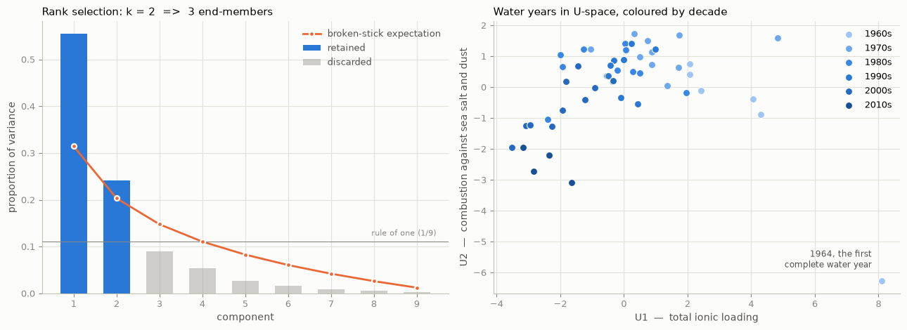
Look at the right-hand panel before reading on. The colours do not form a cloud with three corners. They form a drift: the pale 1960s and 1970s years sit to the upper right, the dark 2000s and 2010s to the lower left, the 1980s and 1990s in between. A mixture of three fixed sources scatters within a triangle; it does not march across one. This is what a system whose sources are changing looks like, and step 5 puts numbers on the march.

(1964, the first complete water year, sits far out on its own. It is the year the full ion suite began, and it is unusually rich in sea salt and dust. It is left in throughout, and flagged rather than deleted.)

Step 5 — Try to pick end-members anyway, and let the diagnostics object

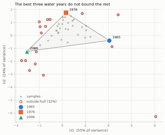
The honest thing is to run the standard procedure and report what it says, rather than stopping because the picture looked wrong. Real measured waters as candidates, screened by how much of the sample cloud they enclose.

ranking = model.suggest_endmembers(years, n_endmembers=3)
ranking.head(5).round(3)

	endmembers	fraction_enclosed	volume
0	1965, 1976, 2006	0.68	9.183
1	1965, 1976, 2009	0.68	10.990
2	1965, 1976, 2008	0.66	9.006
3	1965, 1976, 2011	0.66	10.618
4	1970, 1986, 2012	0.66	12.608

chosen = years.select_rows(ranking.iloc[0]["endmembers"].split(", "))
endmembers = am.EndMembers(chosen.data, chosen.species, tuple(chosen.index))
print(f"the best triangle of all {len(years)} water years encloses "
      f"{model.hull_fraction(chosen):.0%} of them\n")
chosen.to_frame().round(3)

the best triangle of all 50 water years encloses 68% of them

	Ca	Mg	K	Na	NH4	H	SO4	NO3	Cl
1965	0.206	0.049	0.046	0.148	0.209	0.070	3.332	1.395	0.500
1976	0.090	0.022	0.031	0.065	0.170	0.061	2.342	1.796	0.349
2006	0.053	0.016	0.048	0.060	0.113	0.022	1.025	0.773	0.110

fig, ax = plt.subplots(figsize=(6.6, 5.4))
plot_uspace(model, endmembers, ax=ax)
ax.set_title("The best three water years do not bound the rest", loc="left", fontsize=11)
fig.tight_layout()

am.identifiability_report(endmembers, years, model.scores_, model.transform(endmembers))

	value	verdict	note
check
condition number of end-member matrix	6.9	pass	colinear end-members make ratios unstable
closest end-member pair (1965 - 1976)	0.682	pass	relative separation; below 0.2 the pair is eff...
species available vs required	9 vs 2	pass	ne-1 species are the bare minimum; redundancy ...
samples outside the mixing hull (unconstrained solve)	60%	fail	most negative unconstrained ratio -0.967; a mi...
samples enclosed in U-space hull	68%	fail	report this number in every EMMA

Two checks pass and two fail, and the failures are the ones that matter:

• The condition number is 6.9 and the end-members are well separated, so the algebra is fine. A mixing solve would return numbers happily.

• But only 68% of water years fall inside the U-space hull these three define, and on the separate unconstrained check 60% of years need a negative fraction, the worst of them −0.97 — not a rounding error below zero, a fraction that is nonsense by a whole unit.

Per the rule: a negative ratio that large is not a small misfit to be clipped away. It is the conceptual model failing. And look at which years the procedure chose — 1965, 1976 and 2006. Not three sources. Three points strung along the path we just plotted, one early, one middle, one late. The screening had nothing else to offer it.

era = pd.DataFrame(model.scores_, index=annual.index, columns=["U1", "U2"])
era.groupby((era.index // 10) * 10).mean().round(2)

	U1	U2
water_year
1960	3.84	-1.08
1970	1.19	1.13
1980	-0.50	0.59
1990	-0.05	0.52
2000	-1.95	-0.58
2010	-2.49	-2.49

U1 falls from +3.8 in the 1960s to −2.5 in the 2010s, in order apart from a flat patch in the 1980s and 1990s. The “mixing space” is mostly a timeline.

Step 6 — Test the assumption directly

If the sources were fixed and only their proportions changed, then rain from any period would lie in the same low-dimensional subspace. subspace_distance measures exactly that: fit EMMA on one period, ask how far another period’s samples sit from the plane it found.

early = years.select_rows([str(y) for y in range(1964, 1979)])
late = years.select_rows([str(y) for y in range(1999, 2014)])

early_model = am.EMMA(k=2).fit(early)
late_model = am.EMMA(k=2).fit(late)

pd.DataFrame({
    "1964-78 years": [np.median(early_model.subspace_distance(early)),
                      np.median(late_model.subspace_distance(early))],
    "1999-2013 years": [np.median(early_model.subspace_distance(late)),
                        np.median(late_model.subspace_distance(late))],
}, index=["fitted on 1964-78", "fitted on 1999-2013"]).round(2)

	1964-78 years	1999-2013 years
fitted on 1964-78	1.23	4.19
fitted on 1999-2013	6.51	1.33

Read the diagonal against the off-diagonal. Each period sits about 1.2–1.3 from its own subspace and 3 to 5 times further from the other’s. Modern rain is not a different mixture of the same 1960s sources. It is outside the space those sources could produce.

The eigenvectors say the same thing in chemistry:

pd.concat(
    {"1964-78": early_model.loadings_frame().iloc[:, :2],
     "1999-2013": late_model.loadings_frame().iloc[:, :2]},
    axis=1,
).round(2)

	1964-78		1999-2013
	EV1	EV2	EV1	EV2
Ca	0.41	-0.13	0.30	0.21
Mg	0.41	-0.22	0.20	0.48
K	0.40	-0.06	0.06	0.39
Na	0.40	-0.19	0.07	0.51
NH4	0.23	0.53	0.46	-0.10
H	0.27	0.50	0.45	-0.20
SO4	0.32	0.21	0.43	-0.26
NO3	-0.25	0.53	0.46	-0.14
Cl	0.24	0.20	0.21	0.42

The axes have swapped rank. In 1964–78 the leading component is dominated by Ca, Mg, K and Na (+0.40 each) — dust and sea salt were what varied most, and acid rode on the second axis. By 1999–2013 the leading component is NH₄, H⁺, SO₄ and NO₃ (+0.43 to +0.46), and the crustal and marine species have been demoted to the second.

This is the end-member moving. Not the mixing ratios changing — the compositions and the very ranking of the sources changing, inside one continuous record.

Step 7 — What to do instead: an end-member known from outside the data

When the data cannot supply stable end-members, the way forward is an end-member that does not depend on the data at all. Marine aerosol is one: it is seawater, whose composition is known to four figures and has not changed in fifty years.

That converts the problem into a two-component separation per species — marine against everything else — with the marine end-member fixed externally. Conventionally the reference tracer is chloride.

# Seawater mass ratios, S = 35, normalised to chloride.
SEAWATER_PER_CL = {"Na": 0.5571, "Mg": 0.0663, "SO4": 0.1401, "Ca": 0.0213, "K": 0.0206}

marine_cl = pd.DataFrame(
    {s: ratio * annual["Cl"] for s, ratio in SEAWATER_PER_CL.items()}, index=annual.index
)
pd.DataFrame({
    "measured (mg/L)": annual[list(SEAWATER_PER_CL)].mean(),
    "marine share": marine_cl.mean() / annual[list(SEAWATER_PER_CL)].mean(),
}).round(3)

	measured (mg/L)	marine share
Na	0.098	1.330
Mg	0.027	0.567
SO4	1.915	0.017
Ca	0.093	0.054
K	0.048	0.100

A marine share of 1.33 for sodium is impossible — it says more than all of the sodium came from the sea. This is the same failure as a negative mixing ratio, wearing a different hat, and it has the same meaning: an assumption is wrong. The assumption here is that all chloride is marine.

It is not. Coal combustion emits HCl, and 1960s–80s American rain carried a large excess of chloride over the seawater ratio. Chloride is a fine conservative tracer; it is not a conservative marker of marine origin in this system. Sodium is much closer to one.

ratio = (annual["Cl"] / annual["Na"]).rename("Cl/Na by mass")
pd.DataFrame({
    "Cl/Na in rain": ratio.groupby((ratio.index // 10) * 10).mean(),
    "Cl/Na in seawater": 1.0 / SEAWATER_PER_CL["Na"],
}).round(2)

	Cl/Na in rain	Cl/Na in seawater
water_year
1960	3.08	1.8
1970	3.53	1.8
1980	2.23	1.8
1990	1.98	1.8
2000	1.92	1.8
2010	1.69	1.8

There it is. The Cl/Na ratio rises to 3.53 in the 1970s — nearly twice the seawater value — and then falls decade by decade onto it, reaching 1.69 against seawater’s 1.80 by the 2010s. The excess chloride was anthropogenic, it peaked with coal burning, and by the end of the record it is gone. (The last figure sitting a little below seawater is itself informative; see limitation 3.)

That is also the answer to the loose end from step 4: chloride was the one species EMMA called poor because chloride had two sources for most of the record and one by the end. A species whose source membership itself changed cannot be fitted by a model that assumes it did not.

So: redo the separation against sodium.

# The same seawater, normalised to sodium instead.
SEAWATER_PER_NA = {"Cl": 1.7951, "Mg": 0.1191, "SO4": 0.2515, "Ca": 0.0382, "K": 0.0370}

marine = pd.DataFrame(
    {s: ratio * annual["Na"] for s, ratio in SEAWATER_PER_NA.items()}, index=annual.index
)
non_marine = annual[list(SEAWATER_PER_NA)] - marine

pd.DataFrame({
    "measured (mg/L)": annual[list(SEAWATER_PER_NA)].mean(),
    "marine share": marine.mean() / annual[list(SEAWATER_PER_NA)].mean(),
    "non-marine share": non_marine.mean() / annual[list(SEAWATER_PER_NA)].mean(),
}).round(3)

	measured (mg/L)	marine share	non-marine share
Cl	0.234	0.752	0.248
Mg	0.027	0.426	0.574
SO4	1.915	0.013	0.987
Ca	0.093	0.040	0.960
K	0.048	0.075	0.925

Every share is now between 0 and 1. Sulphate is 98.7% non-marine, calcium 96%, potassium 93% — the sea contributes almost nothing to the acid budget, which is what makes the next step meaningful.

Step 8 — The result, and an independent check on it

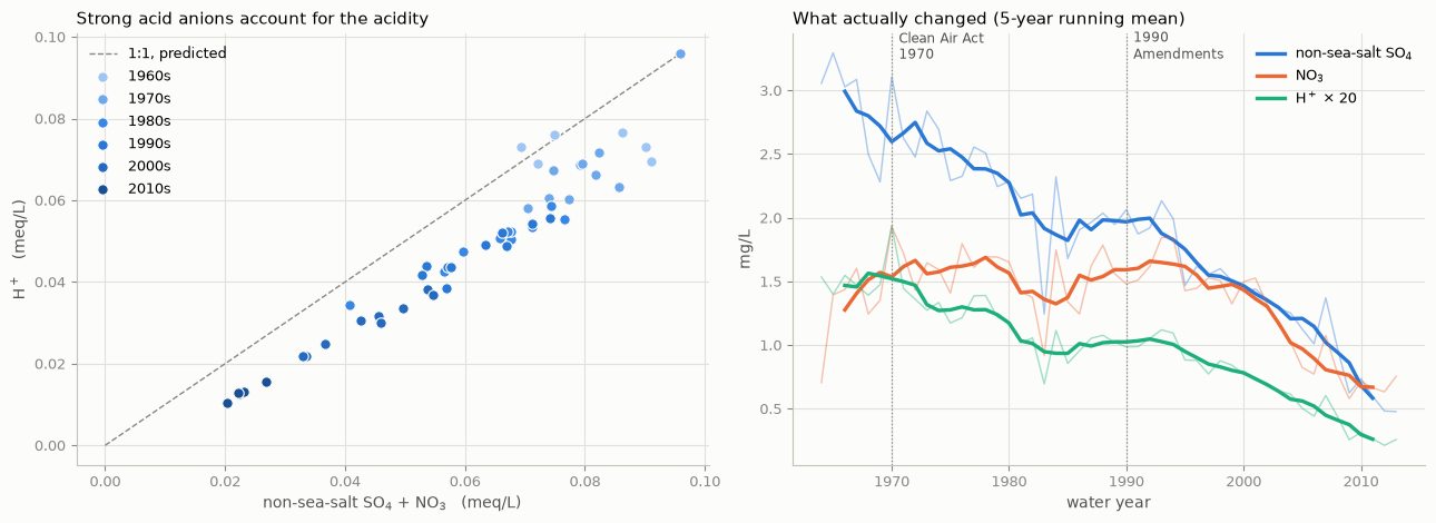
Strong acids dissociate completely. If the acidity of this rain is H₂SO₄ and HNO₃ from combustion, then in milliequivalents the free H⁺ must equal the non-sea-salt sulphate plus the nitrate, one for one, with no fitting. That is a falsifiable prediction, and nothing in the calculation was tuned to make it come out.

# The library already knows these factors, so take them from it rather than
# copying numbers that could drift out of step with the ion table.
from mescla.prep.units import conversion_factors

factors = conversion_factors(["H", "SO4", "NO3"])["factor"]   # 1 / equivalent weight

acid = pd.DataFrame({
    "H": annual["H"] * factors["H"],
    "nssSO4": non_marine["SO4"] * factors["SO4"],
    "NO3": annual["NO3"] * factors["NO3"],
})
acid["strong acid anions"] = acid["nssSO4"] + acid["NO3"]

slope, intercept = np.polyfit(acid["strong acid anions"], acid["H"], 1)
correlation = float(np.corrcoef(acid["strong acid anions"], acid["H"])[0, 1])
print(f"H+ = {slope:.2f} x (nssSO4 + NO3) {intercept:+.4f} meq/L")
print(f"r  = {correlation:.3f}   over {len(acid)} water years")

H+ = 0.96 x (nssSO4 + NO3) -0.0106 meq/L
r  = 0.962   over 50 water years

Slope 0.96 against a predicted 1.00, r = 0.962, across fifty years and a fivefold change in concentration. The small deficit is ammonium, which neutralises a little of the acid before it reaches the collector.

This is what a working mixing result looks like, and it is worth contrasting with step 5. There, the algebra was well conditioned and the answer was meaningless. Here there is no inversion at all — one externally known end-member, one stoichiometric prediction, and an independent check that it holds.

fig, axes = plt.subplots(1, 2, figsize=(13, 4.8))

ax = axes[0]
limit = float(acid["strong acid anions"].max())
ax.plot([0, limit], [0, limit], color=THEME.ink_muted, linewidth=1.0,
        linestyle="--", zorder=1, label="1:1, predicted")
for i, d in enumerate(sorted(decade.unique())):
    mask = np.asarray(decade == d)
    ax.scatter(acid["strong acid anions"].to_numpy()[mask], acid["H"].to_numpy()[mask],
               s=46, color=ramp[i], edgecolor=THEME.surface, linewidth=0.8,
               label=f"{d}s", zorder=3)
ax.set_xlabel("non-sea-salt SO$_4$ + NO$_3$   (meq/L)")
ax.set_ylabel("H$^+$   (meq/L)")
ax.set_title("Strong acid anions account for the acidity", loc="left", fontsize=11)
ax.legend(frameon=False, fontsize=9)
apply_axes_style(ax, THEME)

ax = axes[1]
for i, (name, series) in enumerate([
    ("non-sea-salt SO$_4$", non_marine["SO4"]),
    ("NO$_3$", annual["NO3"]),
    (r"H$^+$ $\times$ 20", annual["H"] * 20),
]):
    ax.plot(annual.index, series, color=series_color(i, THEME), linewidth=1.0, alpha=0.4)
    ax.plot(annual.index, series.rolling(5, center=True).mean(),
            color=series_color(i, THEME), linewidth=2.4, label=name)
for year, label in [(1970, "Clean Air Act\n1970"), (1990, "1990\nAmendments")]:
    ax.axvline(year, color=THEME.ink_muted, linewidth=0.9, linestyle=":")
    ax.annotate(label, (year + 0.6, 3.25), fontsize=8.5, color=THEME.ink_secondary)
ax.set_xlabel("water year")
ax.set_ylabel("mg/L")
ax.set_title("What actually changed (5-year running mean)", loc="left", fontsize=11)
ax.legend(frameon=False, fontsize=9)
apply_axes_style(ax, THEME)

fig.tight_layout()

eras = {"1964-73": (1964, 1973), "1974-83": (1974, 1983), "1984-93": (1984, 1993),
        "1994-2003": (1994, 2003), "2004-13": (2004, 2013)}
summary = pd.DataFrame({
    label: {
        "non-sea-salt SO4 (mg/L)": non_marine.loc[a:b, "SO4"].mean(),
        "NO3 (mg/L)": annual.loc[a:b, "NO3"].mean(),
        "H+ (mg/L)": annual.loc[a:b, "H"].mean(),
        "non-sea-salt Cl (mg/L)": non_marine.loc[a:b, "Cl"].mean(),
        "Na, marine (mg/L)": annual.loc[a:b, "Na"].mean(),
    }
    for label, (a, b) in eras.items()
}).round(3)
summary["last / first"] = (summary.iloc[:, -1] / summary.iloc[:, 0]).map("{:.2f}".format)
summary

	1964-73	1974-83	1984-93	1994-2003	2004-13	last / first
non-sea-salt SO4 (mg/L)	2.829	2.249	1.985	1.525	0.865	0.31
NO3 (mg/L)	1.446	1.516	1.576	1.457	0.782	0.54
H+ (mg/L)	0.074	0.058	0.051	0.041	0.020	0.27
non-sea-salt Cl (mg/L)	0.164	0.088	0.027	0.016	-0.005	-0.03
Na, marine (mg/L)	0.124	0.093	0.085	0.099	0.089	0.72

The combustion-derived species fall by factors of 1.9 (NO₃) to 3.7 (H⁺), and non-sea-salt chloride goes to zero and very slightly past it. Sodium, the marine tracer, falls by only 28% — the weakest trend in the table by some way, and a useful control: whatever happened here was selective, not a general drift in the collectors or the laboratory. Sodium is not perfectly flat, so it is a control with a caveat rather than a constant.

And the acidity, expressed the way it must be — as H⁺, averaged, and only then converted back:

pd.DataFrame({
    "volume-weighted mean H+ (mg/L)": {
        label: annual.loc[a:b, "H"].mean() for label, (a, b) in eras.items()
    },
    "equivalent pH": {
        label: -np.log10(annual.loc[a:b, "H"].mean() / 1008.0)
        for label, (a, b) in eras.items()
    },
}).round(3)

	volume-weighted mean H+ (mg/L)	equivalent pH
1964-73	0.074	4.133
1974-83	0.058	4.237
1984-93	0.051	4.295
1994-2003	0.041	4.392
2004-13	0.020	4.713

pH 4.13 to pH 4.71. Note there is deliberately no ratio column on this table: a ratio of two pH values is meaningless, because pH is a logarithm. The averaging was done on H⁺ and converted afterwards, which is the only correct order.

Conclusion, with its limitations

Result. Bulk precipitation at Hubbard Brook is not describable as a mixture of three fixed sources, and the library’s diagnostics establish that before any ratio is computed: the best triangle of real water years encloses only 68% of the record, an unconstrained solve demands a fraction of −0.97, and each half of the record sits 3–5 times further from the other half’s mixing subspace than from its own. The end-members moved. Between 1964 and 2013 non-sea-salt sulphate fell by a factor of 3.3, nitrate by 1.9, H⁺ by 3.7, and excess chloride disappeared entirely as the Cl/Na ratio fell from 3.5 in the 1970s to 1.7, the seawater value. What can be computed, and checked, is a two-component marine separation against seawater as an externally known end-member: it yields marine shares that are all physically admissible and a stoichiometric prediction, H⁺ = nssSO₄ + NO₃ in meq/L, that the data confirm at slope 0.96 and r = 0.962 without any fitting.

Limitations, in the same breath:

1. Bulk collectors catch dry deposition too, so the “precipitation” here is wet plus an unquantified dry fraction. The crustal component in particular is partly a sampling artefact, and cannot be separated with this dataset alone.

2. One watershed, one site. The EDI package covers nine Hubbard Brook watersheds; the spatial consistency of these end-members is untested here.

3. The marine end-member is assumed unfractionated. Sea-salt aerosol loses chloride to acid displacement during transport, which biases a Cl-referenced correction and is part of why sodium works better — but the sodium reference is not perfect either.

4. suspect is not good. Even at the annual scale, eight of nine species carry RRMSE between 0.09 and 0.26. The three-source picture is a reasonable sketch; it is not a model that would survive being used for prediction.

5. The water-year window (June–May) is a choice, made to match the start of the record. A calendar year or a seasonal split would give somewhat different annual means.

6. Nothing here separates emission reductions from meteorology. The decline is real and its timing matches the 1970 Clean Air Act and its 1990 Amendments, but attribution needs emissions inventories and back-trajectory analysis, not a mixing model.

The general lesson. Notebook 07 said the hardest assumption is that the end-members held still. This record shows what to do when they did not, and it is not to fit a better triangle. It is to find an end-member that comes from outside the data — seawater, a stoichiometry, a mineral formula — and build the separation on that instead. A mixing model with one externally fixed end-member and a testable prediction beat a three-end-member inversion with a perfectly respectable condition number.

The template

import numpy as np
import mescla as am
from mescla.datasets import load_hubbard_brook, load_hubbard_brook_frame

# 1. Never mix pH. Convert to H+ first (the loader does this for you).
samples = load_hubbard_brook()                      # H = 10**-pH * 1.008 * 1000

# 2. Choose the averaging interval so the sources could be constant over it,
#    and weight by the volume that carried the solute.
years = load_hubbard_brook(annual=True)             # volume-weighted water years

# 3. Compare the diagnostics across timescales before choosing k.
am.EMMA(k=2).fit(samples).diagnostics().to_frame()  # monthly: all nine poor
am.EMMA(k=2).fit(years).diagnostics().to_frame()    # annual: one poor

# 4. Before trusting any ratio, ask whether the end-members hold still.
model = am.EMMA(k=2).fit(years)
model.hull_fraction(candidate_endmembers)           # 68% is a failing grade
am.identifiability_report(endmembers, years, ...)   # a -0.97 ratio is a verdict

early, late = years.select_rows(...), years.select_rows(...)
np.median(am.EMMA(k=2).fit(early).subspace_distance(late))   # vs. its own median

# 5. If they do not, replace a data-derived end-member with an external one
#    and make a prediction the data can refute.
non_marine = measured - seawater_ratio * measured_Na
# H+ == nss-SO4 + NO3, in meq/L, with nothing fitted