02 · EMMA: how many source waters, and which species behave as a mixture?

Notebook 01 ended with a suspicion: these waters look like blends of a small number of sources — a salt-affected water, a weathering-dominated water, and the dilute rainwater-derived water both trends run back towards. This notebook turns the suspicion into two answers — how many sources the data require, and which measured species are actually behaving like a conservative mixture. It deliberately stops short of the proportions, which are notebook 03.

Why the number of sources is knowable at all

Take two end-members and blend them in every possible proportion. Plot the results using two tracers, one per axis. Every blend lands on the straight line between the two sources, because each tracer is the same weighted average of its two end-member values. The blends fill a line — a one-dimensional object — no matter how many species you measured.

Now allow three sources. Their blends fill the triangle whose corners are the three sources: a two-dimensional object. Four sources fill a three-dimensional body, and so on. The pattern is worth stating on its own, because the whole of EMMA rests on it:

Blends of n source waters fill a flat region of n − 1 dimensions, with the pure sources at its corners.

So counting sources means counting dimensions of spread in the data and adding one. If a six-species dataset spreads out in only two independent directions, then six measurements are tracing a two-dimensional pattern; two dimensions means a triangle, and a triangle has three corners. Three sources.

Real data never lies exactly in such a region — analytical noise pushes every point a little off it, so strictly the data spreads in as many directions as you have species. The technical content of the next few cells is separating the directions that carry real variation from the ones that carry only noise.

The vocabulary you will meet

EMMA (Christophersen & Hooper, 1992; Hooper, 2003) does the counting with principal component analysis, so its literature uses that vocabulary. Translated into what each thing means here:

term	what it is in this context
principal component	one of the independent directions the data spreads in, found by the method rather than chosen by you
eigenvalue	how much of the spread lies along that direction
loadings	the recipe of species that makes up a direction — this is what tells you what it means chemically
rank, written k	how many of those directions you judge to be real rather than noise. The number of end-members is then k + 1, by the rule in the box above
U-space	the samples redrawn using only the k retained directions as coordinates: a map of the data with the noise dimensions discarded

Nothing below requires you to be comfortable with eigen-decomposition. What it requires is that you read each number as an answer to one of two questions: how many independent directions of variation are there, and what does each of them mean chemically.

import matplotlib.pyplot as plt
import numpy as np
import pandas as pd

import mescla as am
from mescla.datasets import carrera_application2, load_grafton_nh, load_grafton_nh_frame
from mescla.emma.pca import eigen_decomposition
from mescla.plotting import plot_residuals, plot_scree, plot_uspace
from mescla.prep.transform import Standardizer

Part A — the machinery, on data whose answer we already know

A method is best learned on a problem where the truth can be checked afterwards. Carrera et al. (2004)’s Application 2 is synthetic: three end-members, five species, 100 samples, produced by blending known sources in known proportions and adding measurement noise. EMMA is not told any of that, and we compare at the end.

Step 1: put every species on a comparable scale

The directions we are about to look for live in a space whose axes are the measured species, which makes them sensitive to raw magnitude. Bicarbonate near 200 mg/L varies between samples by tens of mg/L; a trace tracer near 0.2 mg/L varies by hundredths. Left as they are, the first would dominate every direction simply by being numerically larger — not by being more informative about sources.

The fix is standardisation: for each species, subtract its mean and divide by its standard deviation across the dataset. Every species then contributes variation of the same size, and the analysis responds to co-variation of pattern rather than to magnitude.

One detail decides whether an EMMA is sound or worthless. The mean and standard deviation must be computed from the mixed samples, and any candidate end-members must then be transformed with those same numbers — never with statistics of their own. Standardising the candidates separately places them in a different coordinate system, after which every figure and diagnostic is meaningless while continuing to look entirely plausible. Standardizer exists so that the correct thing is also the easy thing.

data = carrera_application2(n_samples=100, noise="low", seed=0)

standardizer = Standardizer().fit(data.samples)        # fitted on the SAMPLES
Z = standardizer.transform(data.samples)
Z_endmembers = standardizer.transform(data.endmembers)  # same centre, same scale

print(f"standardised samples: mean {Z.mean():.1e}, sd {Z.std(ddof=1):.4f}")

standardised samples: mean -2.5e-16, sd 0.9960

Step 2: find the directions, and measure the spread along each

This is the principal component analysis. It returns, in order: the direction of greatest spread in the standardised data, then the direction of greatest remaining spread at right angles to the first, and so on, up to the number of species.

Each direction comes with a number — its eigenvalue — giving the amount of the total spread that lies along it. Standardisation gave every species exactly one unit of variation, so the eigenvalues add up to the number of species, and the value 1 acquires a plain meaning: a direction with an eigenvalue of 1 carries one average species’ worth of variation. A direction carrying less than that is contributing less than a single measurement would. The classical criterion, the “rule of one”, is simply to discard those.

eig = eigen_decomposition(Z, data.samples.species)
pd.DataFrame({
    "eigenvalue": eig.eigenvalues.round(4),
    "proportion": eig.explained_variance_ratio.round(4),
}, index=[f"EV{i+1}" for i in range(len(eig.eigenvalues))])

	eigenvalue	proportion
EV1	3.5326	0.7065
EV2	1.4645	0.2929
EV3	0.0012	0.0002
EV4	0.0008	0.0002
EV5	0.0007	0.0001

Two directions carry substantial variation, and then the values fall off a cliff to 0.001. Those later directions are measurement noise and nothing else — which is what we should see, given that the data were built as precise blends of three sources.

So: two dimensions of spread, therefore three end-members. A two-dimensional spread is a triangle, and a triangle has three corners.

Step 3: the number of dimensions is a judgement, so make it in the open

Real data rarely offers a cliff that clean. The rule of one is the oldest criterion and the weakest — it is a rule of thumb resting on a threshold chosen for its tidiness. Mescla reports four criteria side by side so the decision, and any disagreement between the ways of making it, is visible rather than buried:

• rule of one — keep a direction if it carries more than one average species’ worth of variation;

• broken stick — keep it only if it carries more than a random partitioning of the total variation would have handed it by chance;

• parallel analysis — the same idea done by simulation: keep it only if it beats what a table of pure noise of the same size and shape produces;

• cumulative variance — keep however many directions are needed to account for a stated share (90% here) of the total spread.

They are answering slightly different questions, so they can disagree. When they do, that disagreement is a result and should be reported as one.

model = am.EMMA().fit(data.samples)
summary = model.rank_summary()
print("recommended k:", summary.attrs["recommendations"])
print("implied end-members:", summary.attrs["n_endmembers"])
summary.round(4)

recommended k: {'rule_of_one': 2, 'cumulative_variance': 2, 'broken_stick': 2, 'parallel_analysis': 2}
implied end-members: {'rule_of_one': 3, 'cumulative_variance': 3, 'broken_stick': 3, 'parallel_analysis': 3}

	eigenvalue	prop_variance	cum_variance	broken_stick_expected	rule_of_one	cumulative_variance	broken_stick	parallel_analysis
EV1	3.5326	0.7065	0.7065	0.4567	keep	keep	keep	keep
EV2	1.4645	0.2929	0.9994	0.2567	keep	keep	keep	keep
EV3	0.0012	0.0002	0.9997	0.1567
EV4	0.0008	0.0002	0.9999	0.0900
EV5	0.0007	0.0001	1.0000	0.0400

Step 4: the decisive evidence is what the model cannot reproduce

Criteria rank the possibilities; the residuals decide between them. Once you have fixed the number of directions at k, you can project each sample onto that k-dimensional region and convert it back into concentrations — the composition the sample would have if it were exactly a blend. If the picture is right, those reconstructed concentrations match the measured ones to within analytical error, species by species.

Hooper’s (2003) diagnostics report two numbers per species: the relative bias (is this species systematically over- or under-predicted?) and the relative RMSE (how large is the typical misfit, as a fraction of that species’ own variation?). A species the model cannot reproduce is making a specific accusation, and it is worth knowing which: either that species is not conservative in this system, or the number of directions retained is too low, or the end-members are not as constant through time as the method assumes.

model.diagnostics().to_frame().round(4)

	relative_bias	rrmse	verdict
species1	0.0	0.0072	ok
species2	0.0	0.0083	ok
species3	0.0	0.0052	ok
species4	-0.0	0.0060	ok
species5	0.0	0.0099	ok

plot_residuals(data.samples, model.fitted_, n_cols=5);

Structureless clouds scattered about zero, with typical misfits under 1% of each species’ variation. That is what “consistent with blending of three constant sources” looks like. Curvature, a systematic trend against concentration, or one species scattering far wider than the others would each mean the opposite, and would name the species responsible.

Step 5: do the candidate end-members enclose the samples?

Here is a second consequence of the volume-weighted-average rule, and the most useful diagnostic in the method. A blend can never be more extreme than the most extreme water that went into it. Mix a chloride-rich water with a chloride-poor one in any proportion whatsoever and the result lies between the two, never outside.

So on the map of the data — U-space, the samples drawn using the retained directions as coordinates — the end-members have to sit on the outside, with the samples inside the region they enclose: inside the triangle, for three sources. A sample falling outside that region cannot be produced by any blend of those end-members with all proportions positive. It is telling you one of three things: a source is missing from your list, one of your candidate compositions is wrong, or a reaction has moved that sample off the mixing geometry.

hull_fraction is simply the share of samples that fall inside the enclosed region. Report it in every EMMA — it is the one number that says whether the proposed set of sources can account for the data at all.

fig, axes = plt.subplots(1, 2, figsize=(13, 5))
plot_uspace(model, data.true_endmembers, ax=axes[0])
axes[0].set_title("True end-members", loc="left")
plot_uspace(model, data.endmembers, ax=axes[1])
axes[1].set_title("Noisy measured end-members", loc="left")
fig.tight_layout()

print(f"enclosed by the true end-members:    {model.hull_fraction(data.true_endmembers):.0%}")
print(f"enclosed by the measured end-members: {model.hull_fraction(data.endmembers):.0%}")

enclosed by the true end-members:    97%
enclosed by the measured end-members: 85%

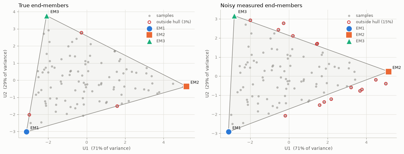
The measured end-members enclose fewer samples than the true ones, because analytical noise has made them less extreme than the sources they stand for. That is systematic rather than bad luck: a noisy measurement of an extreme water is, on average, pulled towards the middle of the cloud, and a corner pulled inwards stops enclosing the points near it. It is one of the arguments for the maximum-likelihood estimator in notebook 04, which uses the fact that the blends themselves contain information about where the corners really are.

Screening candidate waters

If you do have candidate end-members — a sampled spring, a rain collector, an unusually saline well — two tests follow directly from the geometry. A genuine end-member has to be more extreme than the samples it is meant to explain, since otherwise it cannot be a corner; and it has to lie in the same mixing pattern, since otherwise it belongs to a different system altogether. The second is measured as its distance from the k-dimensional region the samples occupy.

model.screen_candidates(data.true_endmembers).round(3)

	extremeness	relative_extremeness	subspace_distance
EM2	5.209	1.037	0.020
EM1	4.349	0.866	0.016
EM3	4.309	0.858	0.013

When you have no candidates at all

Both tools above need candidate waters: screen_candidates scores the ones you supply, and suggest_endmembers picks the best combination of them. Sometimes you have none — no sampled spring, no rain collector, no obviously extreme well.

Archetypal analysis (Cutler & Breiman, 1994) asks the data where the corners would have to be. It looks for k reference compositions such that every sample can be written as a weighted average of them, with weights that are non-negative and add up to one — which is exactly the arithmetic of blending. Imposing that requirement forces the reference compositions out to the edge of the data cloud, because only waters at the edge can average out to the ones in the middle. The geometry that Step 5 above had to check after the fact is here built into what is being optimised.

That is why this, and not a clustering algorithm, is the unsupervised method that belongs in a mixing library. Clustering finds crowded regions, and a crowded region is a commonly observed blend. It is not a source. Sources live at the sparse extremes.

Start with the number of corners. This is a rank criterion of a different kind from the four above: those ask how many directions carry variation, this asks how many corners a region needs in order to enclose the data — which is nearer to the question EMMA is really asking.

am.archetype_rss_curve(data.samples, range(2, 7), n_restarts=5).round(3)

	rss	explained_variance	restarts_at_best	delta_explained
n_archetypes
2	145.843	0.705	1.0	NaN
3	1.320	0.997	1.0	0.292
4	0.836	0.998	0.2	0.001
5	0.916	0.998	0.2	-0.000
6	0.377	0.999	0.2	0.001

Two readings, and the second is the more interesting one.

delta_explained shows the elbow: going from two corners to three buys an enormous amount, and a fourth buys almost nothing. Three corners, agreeing with the eigenvalue criteria.

restarts_at_best is the fraction of random starting points that converge to the best solution found. It sits at 1.0 while the number of corners is right, and collapses as soon as you ask for more corners than the data support — because there is then no well-defined best answer to converge to, and the extra corner can be parked anywhere outside the cloud. The fit is not a convex problem, so this column is a numerical diagnostic and a rank diagnostic at the same time.

Now fit the three:

arch = model.archetypes(seed=0)      # defaults to model.n_endmembers = k + 1
print(arch.summary())

Archetypal analysis: 3 archetypes on 100 samples x 5 species (space='uspace', seed=0)
  explained variance = 99.8% (RSS 0.9606)
  restarts = 10, reaching the best objective = 100%
  converged = True in 18 iterations
  samples effectively supporting each archetype: [1. 1. 1.]
  fraction of samples enclosed = 0.81
  These are candidates, not end-members: name them against the conceptual model first.
  The weights are not mixing ratios -- pass .as_endmembers() to mixing_ratios() or mix_ml().

The summary restates the cautions every time, because they are not optional. Take them in turn against this fit.

The archetypes are recognisably the sources — compare them with the truth we were not allowed to use:

fig, axes = plt.subplots(1, 2, figsize=(13, 5))
plot_uspace(model, data.true_endmembers, ax=axes[0])
axes[0].set_title("True end-members", loc="left")
plot_uspace(model, arch.as_endmembers(), ax=axes[1])
axes[1].set_title("Archetypes, found without being told", loc="left")
fig.tight_layout()

print(f"enclosed by the true end-members: {model.hull_fraction(data.true_endmembers):.0%}")
print(f"enclosed by the archetypes:       {arch.hull_fraction:.0%}")

enclosed by the true end-members: 97%
enclosed by the archetypes:       81%

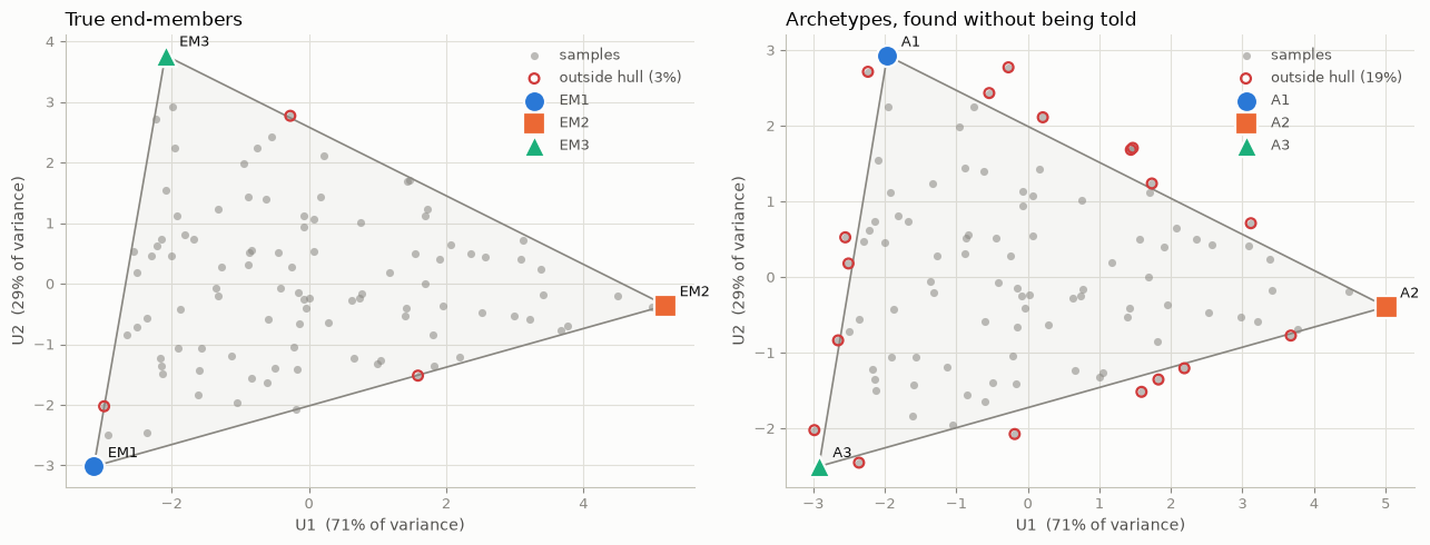
But they are still shrunk inward. The archetypes enclose fewer samples than the true end-members, for exactly the reason the measured end-members did a few cells ago: they are fitted to samples that noise has made less extreme than their sources. Archetypal analysis improves the selection of vertices; it does not do the correction of them. That remains the job of the maximum-likelihood estimator in notebook 04, and this is a second independent argument for it.

Each vertex rests on a handful of real samples. support_frame shows which, and n_effective is roughly how many. A value near 1 means the archetype is one analysis wearing a hat, with all the fragility that implies — the same limitation as choosing a single sample by hand.

And the answer depends on where the optimiser started. A single fit is an anecdote, so refit from different seeds and see whether the vertices come back:

display(arch.support_frame())
am.archetype_stability(data.samples, 3, n_seeds=8, n_restarts=3).round(4)

	n_effective	supporting_samples
archetype
A1	1.029503	S055 (0.99), S002 (0.01)
A2	1.000000	S099 (1.00)
A3	1.000000	S084 (1.00)

	mean_displacement	max_displacement	mean_relative	max_relative
archetype
A1	0.0094	0.0218	0.0019	0.0043
A2	0.0000	0.0000	0.0000	0.0000
A3	0.0000	0.0000	0.0000	0.0000

The one thing this does not give you

The weights are non-negative and add to one, so they look exactly like mixing ratios. They are not, and the library refuses to let that confusion pass silently:

try:
    arch.ratios
except TypeError as err:
    print(err)

archetypal weights are not mixing ratios.
They are reconstruction weights in standardised space: they carry no error model, no per-species sigma, and no distinction between a tracer you trust and one you do not. EMMA and archetypal analysis locate the end-members; they cannot tell you the proportions.
Do this instead:
    ratios = mixing_ratios(result.as_endmembers(), samples, sigma=...)
    ratios = mix_ml(result.as_endmembers(), samples, ...)   # uncertain vertices
If you really want the reconstruction weights, ask for .weights.

Those weights describe how to rebuild a sample from the archetypes in the standardised space of notebook 02’s Step 1 — every species scaled to equal footing, no error model, no per-species uncertainty, no distinction between a tracer you trust and one you do not. Notebooks 03 and 04 compute proportions with all of that taken into account, and they are a separate step for the same reason EMMA and MIX are separate methods.

One last caution, which is about you rather than about the method. Archetypal analysis knows no hydrology. It will return k corners from any data you hand it, whether or not those corners correspond to waters that exist anywhere in the catchment. Use it after the conceptual model is written down — as a check on the candidates it names, or as a starting point when you have none — never as a way of discovering how many sources there are and what they might be. Notebook 07 uses it in exactly that position, on real data, where it agrees with the hand-picked end-members about two sources out of three.

The disagreement there is worth knowing about in advance. suggest_endmembers ranks sets of corners by how many samples they enclose; archetypal analysis instead minimises reconstruction error, and a single very concentrated analysis contributes more of that error than all the ordinary samples together — so the optimiser will spend a corner on it. The two methods can therefore choose different waters, and the archetype set can enclose fewer samples than a hand-picked one. Compare arch.hull_fraction with model.hull_fraction(your_candidates) every time, and read a sharp disagreement as a pointer to the sample the optimiser latched onto rather than as a verdict on either method.

Part B — real data, where the criteria disagree

Now the Grafton County dataset from notebook 01: six species, 130 samples, streams and wells, thirty years of sampling. Nobody knows the answer, and — this is the point of the section — the data will turn out not to satisfy the assumptions at all. Watching the diagnostics say so is more instructive than another clean result.

samples = load_grafton_nh()
real = am.EMMA().fit(samples)
print(real.summary())
print()
real.rank_summary().round(3)

EMMA on 130 samples x 6 species (standardize=True, rule='one')
  retained k = 2 component(s), explaining 76.7% of the variance
  => 3 end-members required
  eigenvalues: [3.344 1.255 0.558 0.386 0.341 0.117]
  species fitting poorly: ['Ca', 'Mg', 'Na', 'K', 'Cl', 'SO4']

	eigenvalue	prop_variance	cum_variance	broken_stick_expected	rule_of_one	cumulative_variance	broken_stick	parallel_analysis
EV1	3.344	0.557	0.557	0.408	keep	keep	keep	keep
EV2	1.255	0.209	0.767	0.242	keep	keep		keep
EV3	0.558	0.093	0.859	0.158		keep
EV4	0.386	0.064	0.924	0.103		keep
EV5	0.341	0.057	0.980	0.061
EV6	0.117	0.020	1.000	0.028

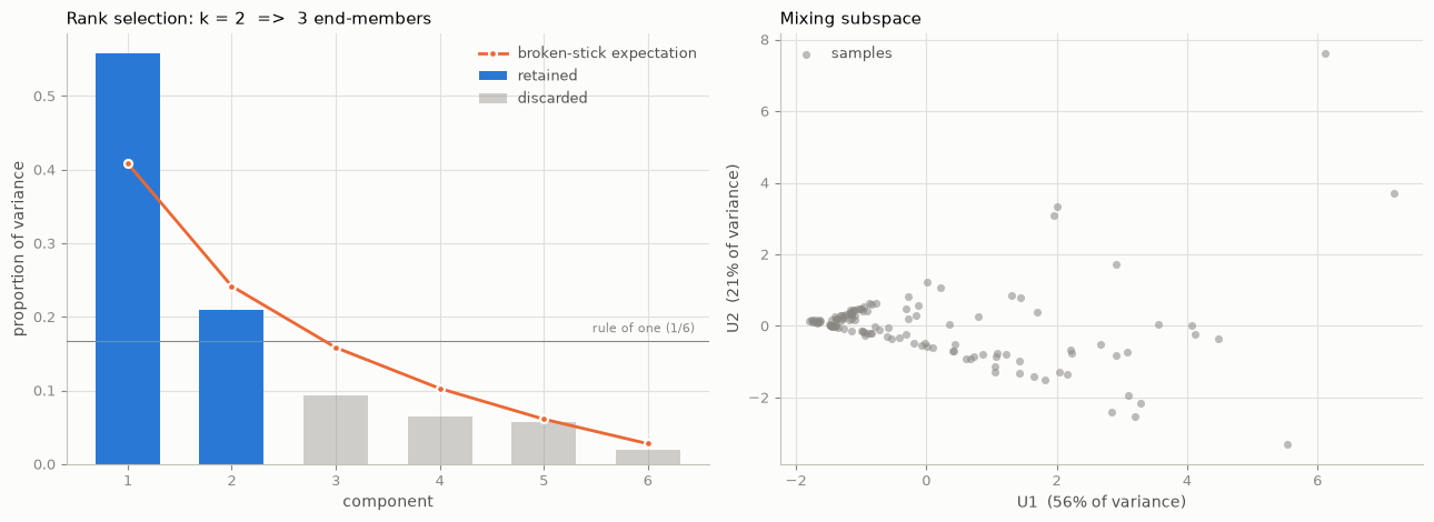
The criteria disagree: the rule of one and parallel analysis say two directions, broken stick says one, cumulative variance at 90% says four. This is normal for real data, and it is why presenting a single criterion as “the” answer is bad practice. Report the disagreement.

What usually settles it is not a rule but chemistry. Each direction has loadings: one number per species, saying how strongly that species contributes to the direction and with which sign. Species with loadings of the same sign rise and fall together along that direction; species with opposite signs trade off against each other. Reading the loadings tells you what process each direction represents, and a direction you can name is a direction worth keeping.

real.loadings_frame().iloc[:, :3].round(3)

	EV1	EV2	EV3
Ca	0.441	-0.268	-0.082
Mg	0.406	-0.255	-0.637
Na	0.399	0.565	0.104
K	0.385	-0.309	0.757
Cl	0.373	0.617	-0.038
SO4	0.441	-0.260	-0.053

Read that table:

• EV1 (56% of the variation): every species loads positive and all by roughly the same amount. Moving along this direction means more of everything at once, which is the dilution/concentration axis — the same water more or less diluted. It is almost always the first component in a hydrochemical EMMA, and it does not discriminate between sources, because every source gets diluted.

• EV2 (21%): sodium (+0.57) and chloride (+0.62) on one side, calcium, magnesium, potassium and sulphate (−0.26 to −0.31) on the other. Samples at one end are rich in Na and Cl and poor in the rest; samples at the other end are the reverse. That is road salt against rock weathering — two genuinely different origins, and it matches the bivariate plots in notebook 01.

The general lesson: the first direction is usually dilution; the science lives in the second and third.

real.diagnostics().to_frame().round(3)

	relative_bias	rrmse	verdict
Ca	0.0	0.680	poor
Mg	-0.0	0.694	poor
Na	0.0	0.353	poor
K	0.0	0.891	poor
Cl	-0.0	0.460	poor
SO4	-0.0	0.398	poor

from mescla.plotting import plot_loadings

plot_loadings(real, n_components=3);

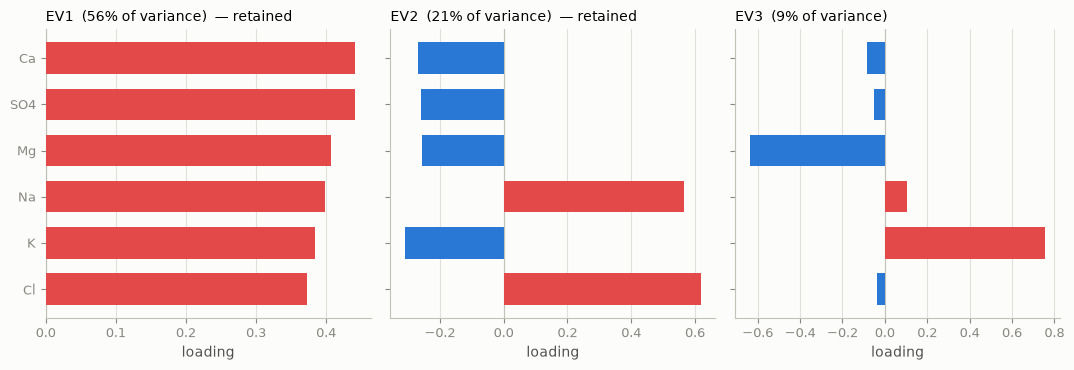
The same table as a figure, which is how you would show it in a talk. EV1 has every species on the same side — dilution. EV2 splits Na and Cl from Ca, Mg, K and SO₄ — road salt against weathering. Tubau et al. (2014) present their analyses A–E exactly this way.

Every species is flagged poor — RRMSE between 0.35 and 0.89. The model is telling us, correctly, that a rank-2 conservative mixing model does not explain this dataset.

That is not a failure of the software; it is the right answer. These 130 samples come from different sites, different water types and thirty years. They are not a mixture of three constant sources, and no amount of fitting will make them one. A well-posed EMMA needs samples from one system with stable end-members — which is the real lesson of this notebook, and why notebook 07 restricts the case study before drawing conclusions.

fig, axes = plt.subplots(1, 2, figsize=(13, 4.8))
plot_scree(real, ax=axes[0])
plot_uspace(real, ax=axes[1])
fig.tight_layout()

Dropping species one at a time

Tubau et al. (2014) work through analyses A–E, removing one species at a time and watching whether the structure simplifies. The reasoning: a species that dominates a direction on its own, without any other species moving with it, is usually reporting a local process — an exchange reaction, a point source — rather than the identity of a source water. If removing it leaves the number of directions and their meaning unchanged, the conceptual model was not resting on it, and that robustness is worth reporting. select_species and drop_species make the experiment a one-liner.

variants = {"all six": samples}
for dropped in ["K", "SO4", "Mg"]:
    variants[f"without {dropped}"] = samples.drop_species(dropped)

rows = []
for name, subset in variants.items():
    fitted = am.EMMA().fit(subset)
    variance = fitted.eigenvalues_[: fitted.k].sum() / fitted.eigenvalues_.sum()
    rows.append({
        "variant": name,
        "species": subset.n_species,
        "k": fitted.k,
        "end-members": fitted.n_endmembers,
        "variance explained": round(variance, 3),
    })
pd.DataFrame(rows).set_index("variant")

	species	k	end-members	variance explained
variant
all six	6	2	3	0.767
without K	5	2	3	0.822
without SO4	5	2	3	0.792
without Mg	5	2	3	0.815

Two directions in every variant: the conceptual model does not depend on which of those three species is included, which is the kind of stability Tubau’s analyses C, D and E were demonstrating. Had the answer flipped when a single species was removed, that species — not the method — would have been deciding the result.

Use this in your own code

import mescla as am

model = am.EMMA().fit(samples)          # samples only -- never include the candidates,
                                        # or they define the space they are tested against

print(model.summary())
model.rank_summary()                    # all four criteria, shown side by side
model.loadings_frame()                  # what each direction MEANS
model.diagnostics().to_frame()          # per-species bias and misfit
model.residual_structure()              # formal test for structure in the residuals

model.screen_candidates(candidates)     # extremeness + distance from the mixing pattern
model.suggest_endmembers(candidates)    # which combination encloses the samples best
model.hull_fraction(chosen)             # REPORT THIS NUMBER

# Force a number of directions you can defend from the loadings rather than from a rule:
model = am.EMMA(k=2).fit(samples)

Next: 03_mixing_ratios_least_squares.ipynb — the proportions themselves.