03 · Mixing ratios: how much of each source is in each sample
EMMA counted the sources and helped identify them. Now comes the question you actually wanted answered: for each sample, what proportion of its volume came from each end-member?
The arithmetic is a direct restatement of the volume-weighted-average rule from notebook 01. For sample p and species s:
Read it as: the measured concentration \(y_{ps}\) equals the sum, over the end-members \(e\), of each end-member’s concentration \(x_{es}\) weighted by the fraction \(\lambda_{pe}\) of that end-member present in the sample, plus a residual \(\varepsilon_{ps}\) that absorbs measurement error and any imperfection in the model. The end-member concentrations are known (that is what notebook 02 was for); the fractions \(\lambda\) are the unknowns.
Every measured species gives one equation like this, so with several tracers you have more equations than unknowns and you solve them together, in a least-squares sense — no single tracer decides the answer alone. The counting rule behind that: with n end-members there are n fractions, but requiring them to add to one uses up one degree of freedom, so n − 1 remain free and you need at least n − 1 tracers that vary independently. Independence is the operative word. Chloride, sodium and electrical conductivity in a salinity-driven system are one tracer measured three times, not three tracers, and they will not resolve three sources.
The two constraints are not decoration:
the fractions add to one, because the sample consists entirely of the listed sources — nothing else contributed volume;
the fractions are non-negative, because you cannot subtract a source from a blend.
A solver that quietly returns −0.3 has not made a small numerical error. It has told you the sample is not a blend of these sources — the same message the enclosing-region check gave in notebook 02, arriving here as a number instead of a picture.
import matplotlib.pyplot as plt
import numpy as np
import pandas as pd

import mescla as am
from mescla.datasets import carrera_application2, make_mixture
from mescla.mixing.geometric import three_component, two_component, uspace_solve
from mescla.plotting import plot_mixing_line, plot_ratios, plot_ternary
The two-component case, worth doing by hand
With two end-members and one tracer there is a closed form, and it is worth keeping in your head because it explains every surprise the general solver will ever hand you. If the sample has concentration \(C_s\) and the two sources are at \(C_1\) and \(C_2\), the fraction of source 1 is
— how far along the way from source 2 to source 1 the sample sits. Two consequences follow immediately. The denominator is the contrast between the sources, so the more alike they are, the more a small analytical error in \(C_s\) swings the answer; contrast, not precision, is usually what limits a mixing study. And a sample lying outside the interval between \(C_2\) and \(C_1\) gives a fraction outside [0, 1].
print("halfway between them:", two_component(50.0, c_1=100.0, c_2=0.0))
print("at end-member 1:      ", two_component(100.0, c_1=100.0, c_2=0.0))
print("beyond end-member 1:  ", two_component(150.0, c_1=100.0, c_2=0.0))
halfway between them: 0.5
at end-member 1:       1.0
beyond end-member 1:   1.5
Three sources, two tracers
Add a second tracer and a third source becomes resolvable. Each sample is now a point on a plane, the three sources are the corners of a triangle, and the fractions answer “whereabouts in this triangle does the sample sit?” — expressed as the weights that make the three corners average out to it. Formally there are three equations (one mass balance per tracer, plus the requirement that the fractions add to one) and three unknowns, so the solution is exact.
endmembers = np.array([[0.0, 0.0], [100.0, 0.0], [0.0, 100.0]])   # 3 end-members x 2 tracers
samples = np.array([[25.0, 25.0], [50.0, 50.0], [10.0, 5.0], [60.0, 60.0]])

pd.DataFrame(
    three_component(samples, endmembers).round(3),
    columns=["EM1", "EM2", "EM3"],
    index=["centre-ish", "on the far edge", "near EM1", "outside"],
)
| EM1 | EM2 | EM3 | |
|---|---|---|---|
| centre-ish | 0.50 | 0.25 | 0.25 |
| on the far edge | 0.00 | 0.50 | 0.50 |
| near EM1 | 0.85 | 0.10 | 0.05 |
| outside | -0.20 | 0.60 | 0.60 |
The general solver
For any number of end-members and species, mixing_ratios solves the same problem by
weighted least squares subject to those two constraints — equation 9 of Carrera et al.
(2004). Two structural facts make it cheap:
when every sample shares the same species and the same assumed errors, the matrix that has to be inverted is identical for every sample, so it is factorised once and reused for all of them;
the problem is well behaved enough that negative fractions can be repaired the simplest possible way — set the most negative fraction to zero, re-solve with it held there, repeat until none are negative — instead of calling a general-purpose constrained optimiser.
It is exact when the data are exact
data = make_mixture(n_endmembers=3, n_species=5, n_samples=40, seed=1)
clean = am.WaterChemistry(data.true_samples, data.samples.species)

exact = am.mixing_ratios(data.true_endmembers, clean)
print(f"worst error against the known truth: {np.abs(exact.ratios - data.true_ratios).max():.2e}")
worst error against the known truth: 3.00e-15
Machine precision. Any implementation that cannot do this is broken, which is why it is the first test in the suite.
With realistic noise
noisy = am.mixing_ratios(data.endmembers, data.samples)
error = np.abs(noisy.ratios - data.true_ratios)
print(f"mean absolute error: {error.mean():.4f}")
print(f"worst sample:        {error.max():.4f}")
print(noisy.diagnostics)
mean absolute error: 0.1259
worst sample:        0.3504
{'n_active_constraints': 17, 'samples_with_active_constraints': 17, 'weighted': True, 'n_missing_analyses': 0, 'n_censored_analyses': 0}
Weighting: telling the estimator which tracers to trust
With more tracers than unknowns the equations will generally disagree a little, and
something has to decide whose version of the answer prevails. That is sigma: the standard
deviation you assign to each measurement, meaning “this number could plausibly be off by
about this much”. A precise, reliably conservative tracer gets a small sigma and effectively
dictates the result; a suspect one gets a large sigma and is carried along without driving
anything.
Sigma is not only instrument precision. If you believe potassium exchanges with clays along
the flow path, its measurement may be excellent while its agreement with a mixing model is
poor — and sigma is where that belief enters the calculation. Guidance on choosing values is
in the assigning-sigma guide; notebook 04 goes further and treats the end-members
themselves as uncertain.
Here two tracers disagree outright. Watch the answer follow the weighting:
em = am.EndMembers([[0.0, 0.0], [100.0, 100.0]], species=["good", "bad"], index=["A", "B"])
sample = am.WaterChemistry([[20.0, 80.0]], species=["good", "bad"])

for label, sigma in [
    ("trust 'good'", [[0.1, 100.0]]),
    ("trust 'bad'", [[100.0, 0.1]]),
    ("trust both equally", None),
]:
    fraction = am.mixing_ratios(em, sample, sigma=sigma).ratios[0, 1]
    print(f"{label:22s} -> fraction of B = {fraction:.2f}")
trust 'good'           -> fraction of B = 0.20
trust 'bad'            -> fraction of B = 0.80
trust both equally     -> fraction of B = 0.50
Unweighted least squares splits the difference at 0.50, which is the wrong answer when you know one of the two tracers is unreliable — it is the right answer only to the question “what if both are equally good?”. Sigma is not a formality. It is where your chemical judgement enters the calculation, and leaving it out is itself a strong assumption rather than a neutral default.
outside = 1.6 * data.true_endmembers.data[0] - 0.6 * data.true_endmembers.data[1]
probe = am.WaterChemistry(outside[None, :], data.samples.species)

free = am.mixing_ratios(data.true_endmembers, probe, non_negative=False)
held = am.mixing_ratios(data.true_endmembers, probe)

print("unconstrained:", free.ratios.round(3))
print("constrained:  ", held.ratios.round(3))
print("active constraints:", held.diagnostics["n_active_constraints"])
unconstrained: [[ 1.6 -0.6  0. ]]
constrained:   [[1. 0. 0.]]
active constraints: 2
The geometry and the algebra are the same thing
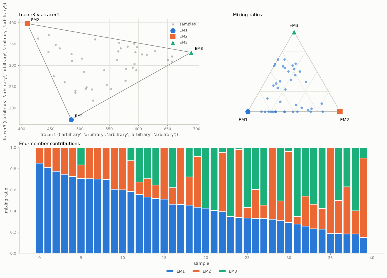
Worth seeing once, because it ties the two notebooks together. Notebook 02 drew the samples on a map and said the end-members are the corners of the region enclosing them. This notebook solves equations for proportions. They are the same operation seen from two sides: a sample’s position inside the triangle of end-members, written as weights on the three corners, is its set of mixing fractions. Computed either way, the numbers agree to machine precision.
clean_samples = am.WaterChemistry(data.true_samples, data.samples.species)
model = am.EMMA(k=2).fit(clean_samples)

from_geometry = uspace_solve(model.scores_, model.transform(data.true_endmembers))
from_algebra = am.mixing_ratios(data.true_endmembers, clean_samples).ratios

print(f"largest disagreement between the two routes: {np.abs(from_geometry - from_algebra).max():.2e}")
largest disagreement between the two routes: 2.89e-15
Figures
result = am.mixing_ratios(data.endmembers, data.samples)
species = data.samples.species

fig = plt.figure(figsize=(13, 9))
ax1 = fig.add_subplot(2, 2, 1)
plot_mixing_line(data.samples, data.true_endmembers, (species[0], species[2]), ax=ax1)
ax2 = fig.add_subplot(2, 2, 2)
plot_ternary(result, ax=ax2)
ax3 = fig.add_subplot(2, 1, 2)
plot_ratios(result, ax=ax3, order_by=0)
fig.tight_layout()
Use this in your own code
import mescla as am

# Weighted by your own judgement of each tracer -- this is the important argument.
sigma = np.column_stack([
    0.03 * samples.data[:, 0],     # Cl: precise and conservative
    0.05 * samples.data[:, 1],     # Na: good
    0.30 * samples.data[:, 2],     # K:  exchanges with clays -- do not let it drive the fit
])
result = am.mixing_ratios(endmembers, samples, sigma=sigma)

result.ratios_frame().to_csv("ratios.csv")
result.mean_ratios()                                   # average contribution per source
result.diagnostics["samples_with_active_constraints"]  # how many sat outside the hull

# Always run this as a check:
free = am.mixing_ratios(endmembers, samples, non_negative=False)
print("most negative unconstrained ratio:", free.ratios.min())
Next: 04_mix_maximum_likelihood.ipynb — what to do when the end-members themselves
are uncertain, which is almost always.