04 · MIX: when the end-members are uncertain

Carrera, J., Vázquez-Suñé, E., Castillo, O. and Sánchez-Vila, X. (2004). A methodology to compute mixing ratios with uncertain end-members. Water Resources Research 40, W12101. (A copy is in papers/.)

Least squares assumes the end-members are known exactly. They almost never are. Their uncertainty comes from spatial and temporal variability and from conceptual error — you often cannot sample a pure end-member at all, and when you can, it changes between campaigns. Mixed samples, by contrast, carry mostly analytical error, which is small.

That asymmetry is the whole idea: the mixtures contain information about the end-members. MIX estimates mixing ratios and end-member compositions jointly, maximising

\[\ln L = \sum_s -\tfrac{1}{2}(z_s - \mu_s)^T A_s^{-1}(z_s - \mu_s)\]

subject to the mixing equations and the simplex constraints, where \(z_s\) stacks every analysis of species \(s\) — end-members first, then samples — and \(A_s\) is its covariance.

The consequence that matters: because all samples are used together, MIX improves as samples accumulate. Least squares, which treats each sample independently, cannot.

import matplotlib.pyplot as plt
import numpy as np
import pandas as pd

import mescla as am
from mescla.datasets import carrera_application1, carrera_application2, load_tubau_besos
from mescla.mixing.ml import improvement_index, mix_ml, profile_objective
from mescla.plotting.theme import LIGHT, apply_axes_style

The claim, tested

Application 2 of the paper: three end-members, five species, noisy end-member analyses (sd 25–100) and precise mixtures (sd 4). We sweep the number of samples and compare.

This takes a minute — it is the paper’s experiment, repeated.

rows = []
for n_samples in [4, 10, 20, 50, 100]:
    for noise in ["low", "high"]:
        for seed in range(4):
            data = carrera_application2(n_samples=n_samples, noise=noise, seed=seed)
            for name, result in [
                ("MIX", mix_ml(data.endmembers, data.samples)),
                ("least squares", am.mixing_ratios(data.endmembers, data.samples)),
            ]:
                rows.append({
                    "n_samples": n_samples,
                    "end-member noise": noise,
                    "method": name,
                    "correlation": np.corrcoef(result.ratios.ravel(), data.true_ratios.ravel())[0, 1],
                    "mean |error|": np.abs(result.ratios - data.true_ratios).mean(),
                })

sweep = pd.DataFrame(rows)
table = sweep.groupby(["end-member noise", "n_samples", "method"])[["correlation", "mean |error|"]].median()
table.round(4)

			correlation	mean |error|
end-member noise	n_samples	method
high	4	MIX	0.9786	0.0440
		least squares	0.9415	0.0688
	10	MIX	0.9733	0.0537
		least squares	0.9125	0.0772
	20	MIX	0.9821	0.0344
		least squares	0.8720	0.0913
	50	MIX	0.9817	0.0366
		least squares	0.9030	0.0737
	100	MIX	0.9900	0.0283
		least squares	0.9036	0.0795
low	4	MIX	0.9956	0.0198
		least squares	0.9876	0.0350
	10	MIX	0.9905	0.0302
		least squares	0.9743	0.0438
	20	MIX	0.9909	0.0245
		least squares	0.9622	0.0522
	50	MIX	0.9902	0.0252
		least squares	0.9691	0.0430
	100	MIX	0.9958	0.0179
		least squares	0.9718	0.0422

fig, axes = plt.subplots(1, 2, figsize=(13, 4.6), sharex=True)
for ax, noise in zip(axes, ["low", "high"]):
    block = sweep[sweep["end-member noise"] == noise]
    for colour, method in zip(LIGHT.series, ["MIX", "least squares"]):
        curve = block[block.method == method].groupby("n_samples")["correlation"].median()
        ax.plot(curve.index, curve.values, marker="o", markersize=7, linewidth=2,
                color=colour, markeredgecolor=LIGHT.surface, markeredgewidth=1.6, label=method)
    ax.set_xscale("log")
    ax.set_xticks([4, 10, 20, 50, 100]); ax.set_xticklabels([4, 10, 20, 50, 100])
    ax.set_xlabel("number of mixed samples")
    ax.set_ylabel("correlation with the true ratios")
    ax.set_title(f"{noise} end-member noise", loc="left", fontsize=11)
    apply_axes_style(ax, LIGHT)
axes[0].legend(frameon=False, fontsize=9)
fig.tight_layout()

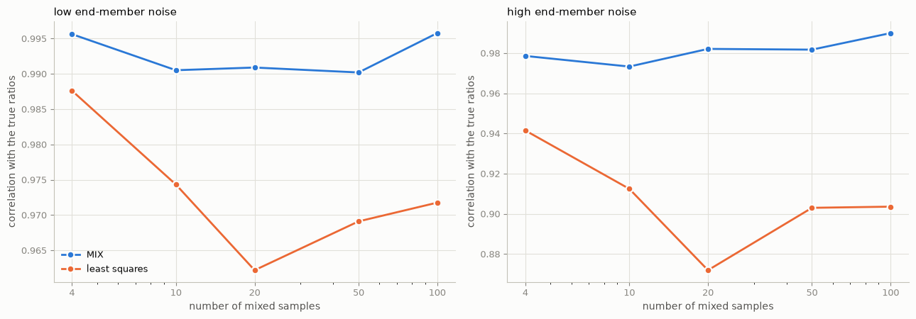
Read the right-hand panel carefully. It contains the paper’s central result:

• MIX rises with sample count. More mixtures teach it more about the sources, so its estimate of both improves.

• Least squares is flat or drifts down. It estimates each sample in isolation, so it literally cannot benefit from the others.

• MIX is nearly insensitive to end-member noise once there are enough samples, while least squares degrades sharply — compare the two panels.

The published bands are reproduced: least-squares correlations of 0.97–0.98 at low end-member noise and 0.93–0.94 at high noise. These are assertions in tests/test_reproduce_carrera2004.py, not just claims in a notebook.

The end-members themselves get better

That is the other half of the method. The improvement index (the paper’s equation 28) is the ratio of prior to posterior mean square error of the end-member concentrations: IM = 2 means the error was halved.

It can only be computed when the truth is known, so it is a validation diagnostic.

rows = []
for n_samples in [4, 10, 20, 50, 100]:
    values = []
    for seed in range(5):
        data = carrera_application2(n_samples=n_samples, noise="low", seed=seed)
        fit = mix_ml(data.endmembers, data.samples)
        values.append(improvement_index(fit.endmembers.data, data.true_endmembers.data,
                                        data.endmembers.sigma))
    rows.append({"n_samples": n_samples, "improvement index": np.median(values)})
pd.DataFrame(rows).set_index("n_samples").round(2)

	improvement index
n_samples
4	6.22
10	4.25
20	6.78
50	8.63
100	6.49

Between about 4 and 10 — the paper reports a rise from 3 with four samples to 8 with a hundred. Our medians sit in the same band. The end-member compositions are several times more accurate after estimation than the analyses that went in.

Watch it move an end-member

data = carrera_application2(n_samples=100, noise="high", seed=1)
fit = mix_ml(data.endmembers, data.samples)

comparison = pd.DataFrame({
    "true": data.true_endmembers.data[0],
    "measured": data.endmembers.data[0],
    "estimated by MIX": fit.endmembers.data[0],
}, index=data.samples.species)
comparison["measured error"] = (comparison["measured"] - comparison["true"]).abs()
comparison["MIX error"] = (comparison["estimated by MIX"] - comparison["true"]).abs()
comparison.round(1)

	true	measured	estimated by MIX	measured error	MIX error
species1	500.0	479.7	456.5	20.3	43.5
species2	700.0	178.2	752.3	521.8	52.3
species3	100.0	-33.2	-61.1	133.2	161.1
species4	800.0	976.8	855.4	176.8	55.4
species5	200.0	225.8	233.6	25.8	33.6

The part that decides your answer: assigning sigma

MIX needs a standard deviation for every species in every end-member and every sample. Results are robust to moderate misspecification, but the relative weighting between end-members and samples is a real modelling decision — and it points in different directions at different stages:

stage	which sigma is larger	why
estimating end-members from the mixtures	end-member sigma > sample sigma	you want the mixtures to reshape the end-members
end-members already established, fitting new samples	sample sigma > end-member sigma	you do not want new data to undo the previous fit

Tubau et al. (2014) do exactly this: loose end-members in the river step, tight ones in the groundwater step. Here is the same data fitted three ways.

data = carrera_application2(n_samples=60, noise="high", seed=2)

schemes = {
    "end-members loose (x5)":  (5.0 * data.endmembers.sigma, data.samples.sigma),
    "as measured (x1)":        (data.endmembers.sigma, data.samples.sigma),
    "end-members tight (x0.1)": (0.1 * data.endmembers.sigma, data.samples.sigma),
}

rows = []
for label, (sd_e, sd_y) in schemes.items():
    fit = mix_ml(data.endmembers, data.samples, sd_endmembers=sd_e, sd_samples=sd_y)
    rows.append({
        "sigma scheme": label,
        **{f"mean {k}": v for k, v in zip(data.endmembers.labels, fit.ratios.mean(axis=0).round(3))},
        "error vs truth": round(float(np.abs(fit.ratios - data.true_ratios).mean()), 4),
        "end-members moved (sigmas)": round(float(np.abs(fit.diagnostics["endmember_shift_in_sigmas"]).mean()), 2),
    })
pd.DataFrame(rows).set_index("sigma scheme")

	mean EM1	mean EM2	mean EM3	error vs truth	end-members moved (sigmas)
sigma scheme
end-members loose (x5)	0.327	0.343	0.331	0.0268	0.11
as measured (x1)	0.323	0.349	0.327	0.0222	0.47
end-members tight (x0.1)	0.307	0.356	0.337	0.0263	4.32

Same data, three answers. Declaring the end-members tight pins them where they were measured — which, since they were measured badly, is the worst result. Declaring them loose lets the mixtures pull them towards the truth.

So sweep it, and report the sweep. sigma_sweep does this in one call; notebook 05 uses it.

A published sigma scheme, with all its strangeness

load_tubau_besos() ships the actual standard deviations from Tubau et al. (2014) — the best-documented published example of this judgement.

besos = load_tubau_besos()
besos.table[["species", "sd_factor_endmember", "sd_factor_river",
             "sd_factor_groundwater", "conservative"]].head(14)

	species	sd_factor_endmember	sd_factor_river	sd_factor_groundwater	conservative
0	Cl	0.04	0.05	0.05	yes
1	EC	0.03	0.07	0.07	yes
2	Na	0.05	0.07	0.07	yes
3	SO4	0.04	0.12	0.11	yes
4	HCO3	0.07	0.11	0.10	no
5	Ca	0.06	0.19	0.16	no
6	Mg	0.10	0.37	0.28	no
7	K	0.17	0.50	0.79	no
8	Ntot	0.12	0.43	1.00	no
9	NO3	0.47	5.54	15.00	no
10	NH4	0.12	0.40	0.90	no
11	P	0.48	7328.00	27756.00	no
12	PO4	0.70	29758.00	125434.00	no
13	F	0.57	14193.00	11342.00	no

The factors are fractions of the mean river concentration. Note their range:

• Conservative species (Cl, EC, Na, SO₄) get 0.03–0.12. Tight: these drive the fit.

• Reactive major ions (Ca, Mg, K, NH₄) get 0.16–0.79. Loose.

• NO₃ gets 5.5 in the river and 15 in the groundwater — larger than the concentration itself. The authors decided explicitly not to explain nitrate, because it is redox-active.

• Trace and data-poor species (P, PO₄, F, TOC, As, Br, B, O₂, Fe) get factors of thousands to over a hundred thousand.

Those last ones are not typos. They are the published device for carrying a species through the calculation so its end-member composition is predicted, without letting it influence the fit at all. You get a free estimate of the composition of species you barely measured. It is an elegant trick and worth reusing.

besos.endmembers.to_frame().T.round(3)

	W1	D1	D2
Cl	43.700	356.200	315.800
EC	585.600	1996.500	1891.500
Na	29.000	280.900	246.600
SO4	52.800	205.900	198.600
HCO3	222.700	500.500	470.300
Ca	62.200	133.900	151.300
Mg	13.200	24.200	30.100
K	7.200	51.100	36.400
Ntot	6.200	26.100	5.700
NO3	13.400	7.400	13.200
NH4	4.100	31.500	3.600
P	0.000	2.305	2.012
PO4	1.904	3.818	3.177
F	0.187	1.244	0.374
TOC	6.323	12.427	8.663
As	0.003	0.006	0.008
Br	0.059	0.570	0.854
B	0.034	0.218	0.292
O2	8.736	8.267	10.601
Fe	0.036	0.209	0.232

W1 is wet-period river water — dilute in everything but the nitrogen species. D1 and D2 are dry-period waters, separated mainly by ammonium against calcium and magnesium. Published result: the dry-season end-members dominate the wet one in the aquifer — D2 65%, W1 26%, D1 9%. (The paper’s prose says “4:1”; its own percentages give 2.8:1. We follow the percentages.)

Checking the implementation against the paper’s own formulation

The paper eliminates the concentrations analytically and solves the remaining nonlinear system by Newton–Raphson. Mescla instead carries them as explicit unknowns and alternates two closed-form steps — block coordinate descent on the same likelihood.

Those are only equivalent if the objectives agree, so we check rather than assert. profile_objective implements the paper’s eliminated objective (equation 21) directly.

data = carrera_application2(n_samples=60, noise="low", seed=0)
fit = mix_ml(data.endmembers, data.samples)

eliminated = profile_objective(
    fit.ratios, data.endmembers.data, data.samples.data,
    data.endmembers.sigma ** 2, data.samples.sigma ** 2,
)
print(f"block coordinate descent objective : {fit.objective:.8f}")
print(f"paper's eliminated objective (eq 21): {eliminated:.8f}")
print(f"difference: {abs(fit.objective - eliminated):.2e}")

block coordinate descent objective : 97.86483429
paper's eliminated objective (eq 21): 97.86483429
difference: 6.68e-13

Identical to eight decimals. This is also an assertion in the test suite.

One practical note the docstring records: the alternation has a long, very flat tail. The objective can creep in the sixth decimal for thousands of iterations after the ratios have settled to better than 1e-4 — already far beyond analytical precision. So converged reports whether both movement criteria were met, and you should read diagnostics["final_ratio_change"] rather than the flag alone.

print(f"converged flag:      {fit.converged}")
print(f"iterations:          {fit.diagnostics['iterations']}")
print(f"final ratio movement: {fit.diagnostics['final_ratio_change']:.2e}   <- this is what matters")
print(f"restarts tried:      {fit.diagnostics['n_starts']}")

converged flag:      False
iterations:          2030
final ratio movement: 1.17e-05   <- this is what matters
restarts tried:      12

Multiple restarts are not decoration: the paper explicitly reports converging to different minima from different starting points, and recommends trying least squares, uniform and about ten random perturbations, then keeping the best. Mescla does that.

When not to use MIX

rows = []
for n_samples in [4, 6, 10]:
    mix_errors, lsq_errors = [], []
    for seed in range(8):
        data = carrera_application2(n_samples=n_samples, noise="low", seed=seed)
        mix_errors.append(np.abs(mix_ml(data.endmembers, data.samples).ratios - data.true_ratios).mean())
        lsq_errors.append(np.abs(am.mixing_ratios(data.endmembers, data.samples).ratios - data.true_ratios).mean())
    rows.append({"n_samples": n_samples,
                 "MIX": round(float(np.median(mix_errors)), 4),
                 "least squares": round(float(np.median(lsq_errors)), 4)})
pd.DataFrame(rows).set_index("n_samples")

	MIX	least squares
n_samples
4	0.0247	0.0446
6	0.0283	0.0456
10	0.0304	0.0420

With only a handful of samples the advantage is small or absent — the paper says the same, and notes that MIX can even produce negative end-member concentrations there. Its benefit comes from redundancy. Few samples and well-known end-members: use least squares.

Use this in your own code

from mescla import MixML, mix_ml

result = mix_ml(
    endmembers, samples,
    # LOOSE: conceptual and temporal variability, not laboratory precision
    sd_endmembers=0.30 * endmembers.data,
    # TIGHT: analytical error on the mixtures
    sd_samples=0.05 * samples.data,
)

result.ratios_frame()                       # the mixing ratios
result.endmembers.to_frame()                # the REVISED end-member compositions
result.diagnostics["endmember_shift_in_sigmas"]   # how far each moved, in its own sigma

# Carry a species you do not trust, to get its composition predicted for free:
sd = 0.05 * samples.data
sd[:, samples.species.index("NO3")] *= 1000
result = mix_ml(endmembers, samples, sd_endmembers=0.3 * endmembers.data, sd_samples=sd)

# Estimator form, for pipelines:
model = MixML(sd_endmembers=sd_e, sd_samples=sd_y).fit(endmembers, samples)

Next: 05_uncertainty.ipynb — never report a mixing fraction without one.