01 · Real data, units and quality control

What this series is trying to do

You have water samples — wells, streams, springs — and you suspect each one is a blend of a few distinct source waters: rain that infiltrated recently, older regional groundwater, river water pulled in by pumping, seawater, irrigation return flow. You cannot see underground and you cannot watch the blending happen. All you have is the dissolved chemistry of each sample.

That turns out to be enough, because of one fact. When waters blend, the concentration of a dissolved substance in the blend is the volume-weighted average of the concentrations in the waters that went in. A litre of river water at 200 mg/L chloride plus a litre of groundwater at 20 mg/L gives two litres at 110 mg/L — not 220, not 2000. Read that backwards and the chemistry of a sample becomes a statement about the volumes that made it. Chemistry is the label each water carries out of its source.

Some vocabulary, used consistently from here on:

• an end-member is one of those source waters in its pure, unblended state;

• a mixing ratio (or mixing fraction) is the volume proportion of one end-member in one sample — three sources means three fractions per sample, and they add up to 1;

• a conservative tracer is a dissolved species whose concentration changes only through blending and dilution. Chloride usually qualifies. Nitrate, in a system where bacteria consume it, does not. The volume-weighted average rule holds only for species that are conservative in the system you are studying, which is a judgement about that system and not a property you can look up.

Two questions follow, and they need two different calculations:

	the question it answers	notebook
EMMA	How many end-members does the data require, and which species are behaving as a mixture?	02
Mixing ratios	Given the end-members, what proportion of each is in each sample?	03, 04

Neither one answers the other’s question, and the order matters: you cannot apportion a sample among sources you have not yet counted and identified.

Why this notebook comes first

Both calculations take your numbers at face value. A mixing calculation cannot tell you that an analysis is wrong — it will cheerfully apportion a nonsense sample among your end-members and hand back confident-looking fractions. The checks below cost minutes, they catch the failures that would otherwise be invisible downstream, and they belong at the top of every analysis.

Dataset. 130 complete major-ion analyses (Ca, Mg, Na, K, Cl, SO₄) from 66 stream and 64 groundwater-well samples in Grafton County, New Hampshire — the county containing the Hubbard Brook Experimental Forest — collected 1990–2021. Retrieved from the Water Quality Portal; U.S. Geological Survey data, public domain. Full provenance in src/mescla/datasets/data/SOURCES.md.

import matplotlib.pyplot as plt
import numpy as np
import pandas as pd

import mescla as am
from mescla.datasets import load_grafton_nh, load_grafton_nh_frame
from mescla.prep.qaqc import missing_data_report
from mescla.prep.units import to_meq_per_l, to_mmol_per_l

frame = load_grafton_nh_frame()
print(frame.shape, "samples")
frame.head()

(130, 9) samples

	site	date	site_type	Ca	Mg	Na	K	Cl	SO4
0	USGS-435613071420702	1990-05-09	Well	14.0	4.50	7.9	12.00	7.1	14.0
1	USGS-435613071420703	1990-05-09	Well	2.0	0.37	3.0	0.56	1.8	5.0
2	USGS-435613071420701	1990-05-10	Well	44.0	8.90	7.2	2.90	41.0	14.0
3	USGS-435612071420701	1990-05-15	Well	14.0	3.70	5.3	2.40	0.4	7.4
4	USGS-435612071420702	1990-05-15	Well	5.6	1.00	3.2	1.40	2.7	4.6

The container

WaterChemistry is a matrix plus the labels needed to keep species and samples straight. Every function in the library accepts a plain array, a DataFrame or one of these, so use whichever you happen to have.

samples = load_grafton_nh()
samples

<WaterChemistry: 130 rows x 6 species [mg/L, no sigma]
  species: Ca, Mg, Na, K, Cl, SO4>

samples.to_frame().describe().round(2)

	Ca	Mg	Na	K	Cl	SO4
count	130.00	130.00	130.00	130.00	130.00	130.00
mean	11.60	1.76	5.18	1.53	7.03	7.46
std	15.58	2.03	7.04	2.20	13.60	5.79
min	0.31	0.10	0.29	0.12	0.17	0.27
25%	2.20	0.43	1.80	0.40	0.53	3.81
50%	4.50	0.78	3.30	0.78	2.15	4.78
75%	16.00	2.20	5.78	1.80	5.70	9.05
max	100.00	8.90	54.00	17.00	100.00	29.20

Look at the spread: chloride from 0.17 to 100 mg/L, calcium from 0.31 to 100. That range is the point. A tracer earns its place by differing between the sources, because the whole method works by recognising the sources’ signatures inside a blend. If two sources have the same chloride concentration, then no chloride measurement can ever say which of them a sample came from, however precisely it was measured. Wide ranges are a sign that there is something to resolve; a species that is nearly constant across the dataset carries almost no information about proportions.

Units

Units are per species, and stated rather than assumed. The default is mg/L, which is what every loader returns. A real analysis sheet routinely mixes units, though — concentrations in mg/L beside conductivity in µS/cm and a delta value in permil — so one label for the whole table could only describe such a table by lying about part of it.

print("common unit:", samples.common_unit)       # None when the table mixes units
samples.units_dict()

common unit: mg/L

{'Ca': 'mg/L',
 'Mg': 'mg/L',
 'Na': 'mg/L',
 'K': 'mg/L',
 'Cl': 'mg/L',
 'SO4': 'mg/L'}

Mixing arithmetic happens inside one species at a time — chloride is averaged against chloride, never against sodium — so a table carrying different units in different columns is mathematically harmless here. Multiply every chloride value by a thousand and the mixing fractions come out unchanged.

The conversions still matter, for the checks rather than for the mixing. Two other units appear throughout:

• mmol/L counts particles instead of mass, which is what makes reaction stoichiometry readable: one mole of gypsum dissolving releases one mole of calcium and one of sulphate, a 1:1 relationship that is invisible in mg/L because those moles weigh different amounts;

• meq/L counts charge — millimoles multiplied by the ion’s charge, so 1 mmol/L of Ca²⁺ is 2 meq/L. This is the unit the charge-balance check below is written in, for the reason that section explains.

first = samples.select_rows([samples.samples[0]])
print("mg/L  :", first.to_frame().iloc[0].round(2).to_dict())
print("meq/L :", to_meq_per_l(first).to_frame().iloc[0].round(3).to_dict())
print("mmol/L:", to_mmol_per_l(first).to_frame().iloc[0].round(3).to_dict())

mg/L  : {'Ca': 14.0, 'Mg': 4.5, 'Na': 7.9, 'K': 12.0, 'Cl': 7.1, 'SO4': 14.0}
meq/L : {'Ca': 0.699, 'Mg': 0.37, 'Na': 0.344, 'K': 0.307, 'Cl': 0.2, 'SO4': 0.291}
mmol/L: {'Ca': 0.349, 'Mg': 0.185, 'Na': 0.344, 'K': 0.307, 'Cl': 0.2, 'SO4': 0.146}

What converts, and by what factor

Nothing is hidden. conversion_factors returns exactly the table the conversions read, so you can check that a species was recognised under the name you used — matching ignores case and charge notation, so "Ca", "Ca2+" and "calcium" are the same ion.

from mescla.prep.units import conversion_factors

conversion_factors(samples).round(4)

	matched_ion	molar_mass	charge	equivalent_weight	factor	target_unit	convertible
species
Ca	Ca	40.0780	2	20.0390	0.0499	meq/L	True
Mg	Mg	24.3050	2	12.1525	0.0823	meq/L	True
Na	Na	22.9898	1	22.9898	0.0435	meq/L	True
K	K	39.0983	1	39.0983	0.0256	meq/L	True
Cl	Cl	35.4530	-1	35.4530	0.0282	meq/L	True
SO4	SO4	96.0600	-2	48.0300	0.0208	meq/L	True

A species that cannot convert stops the call

An equivalent weight is molar mass divided by charge, so a neutral species has none, and a species that is not an ion at all has no factor either. Rather than pass such a column through untouched while relabelling the table — which returns something that looks converted and is not — the conversion refuses and asks you to choose.

The Besòs end-members show both problems at once, and they are worth keeping apart:

• mixed units — nineteen species in mg/L and one, electrical conductivity, in µS/cm;

• unconvertible species — seven of the twenty have no equivalent weight, either because they are neutral (TOC, B, O₂) or because they are not single ions at all (EC, N_tot, P, As).

Units and convertibility are different questions. A species can be in mg/L and still have no meq/L to convert to.

from mescla.datasets import load_tubau_besos

besos = load_tubau_besos().endmembers
print("mixed units:", {k: v for k, v in besos.units_dict().items() if v != "mg/L"})

try:
    to_meq_per_l(besos)
except ValueError as error:
    print("\nrefused:\n ", str(error).split("\n\n")[0].replace("\n", "\n "))

mixed units: {'EC': 'uS/cm'}

refused:
  cannot convert to meq/L:
   'EC': not a recognised ion
   'Ntot': not a recognised ion
   'P': not a recognised ion
   'TOC': TOC is neutral, so it has no equivalent weight
   'As': not a recognised ion
   'B': B is neutral, so it has no equivalent weight
   'O2': O2 is neutral, so it has no equivalent weight

Three ways forward, chosen explicitly:

on_unknown	what happens	when
"raise" (default)	refuses, naming the species	you expected everything to convert
"skip"	keeps them with their own unit	the table legitimately holds EC, silica or isotopes
"drop"	removes those columns	you want a purely ionic table

"skip" is honest precisely because units are per species — the result says which columns were converted and which were left alone.

converted = to_meq_per_l(besos, on_unknown="skip")
print("after skip:", {k: converted.unit_of(k) for k in ("Cl", "Na", "EC")})
print("EC value unchanged:", converted.unit_of("EC"), converted.to_frame().loc["W1", "EC"])

dropped = to_meq_per_l(besos, on_unknown="drop")
print(f"\nafter drop: {dropped.n_species} of {besos.n_species} species kept,"
      f" all in {dropped.common_unit}")

after skip: {'Cl': 'meq/L', 'Na': 'meq/L', 'EC': 'uS/cm'}
EC value unchanged: uS/cm 585.6

after drop: 13 of 20 species kept, all in meq/L

charge_balance_report uses "skip" internally, because it deliberately considers only the major ions.

If a loader guessed wrong

with_units relabels without converting — it states what the numbers already are:

samples = samples.with_units({"EC": "uS/cm"})

Where the label actually matters

operation	depends on it?
mixing_ratios, mix_ml, EMMA	no — linear within each species
to_meq_per_l, to_mmol_per_l	yes — decides what is already converted
charge_balance_report, ec_check	yes — they convert internally

So a mislabelled table will not corrupt a mixing ratio, but it will corrupt a charge balance. If your data is already in meq/L, say so when you build the table: WaterChemistry(data, species=[...], units="meq/L").

Charge balance: is the analysis complete?

Water is electrically neutral. Whatever positive charge the dissolved cations carry, the dissolved anions must carry the same amount of negative charge. So if every major ion has been measured, and measured well, the two sums — counted in meq/L, which is why that unit exists — have to agree. When they do not, either something was measured badly or something was not measured at all. That is the whole idea, and it is the standard first test of any water analysis:

\[\mathrm{CBE} = 100\,\frac{\sum \mathrm{cations} - \sum \mathrm{anions}} {\sum \mathrm{cations} + \sum \mathrm{anions}}\]

Conventional acceptance is |CBE| < 5%, relaxed to 10% for very dilute waters, where a small absolute error is a large relative one.

Quote the convention with the number. Two are in circulation and they differ by a factor of two: the default convention="sum" divides by the sum of the two ion sums (Freeze & Cherry; what PHREEQC prints), while convention="mean" divides by their mean (APHA 1030E). The ±5% rule is quoted for both, so the same water can pass one and fail the other. The report records which it used in .attrs["convention"].

These samples will fail badly, and that is the lesson. The dataset has no bicarbonate, and in dilute weathering-dominated waters bicarbonate is the dominant anion. Its absence leaves the cation sum unmatched, so the error comes out large and positive — a missing anion, which is exactly what we have. The check is doing its job.

report = am.charge_balance_report(samples, tolerance=5.0)
print("species used:", report.attrs["species_used"])
print("convention:  ", report.attrs["convention"])
print(f"passing: {report['pass'].sum()} of {len(report)}")
report["cbe_percent"].describe().round(1)

species used: {'cations': ['Ca', 'Mg', 'Na', 'K'], 'anions': ['Cl', 'SO4']}
convention:   sum
passing: 3 of 130

count    130.0
mean      39.0
std       21.9
min       -1.5
25%       23.8
50%       30.8
75%       54.8
max       93.5
Name: cbe_percent, dtype: float64

A median charge-balance error of about +31%, with 3 of 130 samples passing, is a red flag that says “you have not measured all the major ions”, not “these analyses are wrong”. Before doing mixing work on this dataset for real, you would go back for alkalinity. We continue here because the six species are still enough to demonstrate the machinery — but we do so knowingly, which is the difference between a caveat and a mistake.

Missing data

missing_data_report(samples)

	n_missing	fraction_missing
Ca	0	0.0
Mg	0	0.0
Na	0	0.0
K	0	0.0
Cl	0	0.0
SO4	0	0.0

Look at the chemistry before modelling it

Plot two tracers against each other and blending becomes visible directly. If every sample in a group is a blend of the same two sources, each tracer in it is the same weighted average of that tracer’s two end-member values — so the samples fall along the straight line joining the two sources, with the position along the line set by the proportions. Straight-line trends in a bivariate plot are therefore the visual signature of two-component mixing. Curvature means something other than simple blending — a reaction, or a third source. A point sitting far off on its own is usually an analytical error, or a sample that belongs to a different system.

from mescla.plotting.theme import LIGHT, apply_axes_style

streams = frame[frame.site_type == "Stream"]
wells = frame[frame.site_type == "Well"]

fig, axes = plt.subplots(1, 3, figsize=(15, 4.4))
for ax, (x, y) in zip(axes, [("Cl", "Na"), ("Ca", "Mg"), ("Cl", "SO4")]):
    ax.scatter(streams[x], streams[y], s=28, c=LIGHT.series[0], alpha=0.75, label="stream")
    ax.scatter(wells[x], wells[y], s=28, c=LIGHT.series[1], alpha=0.75, label="well")
    ax.set_xscale("log"); ax.set_yscale("log")
    ax.set_xlabel(f"{x} (mg/L)"); ax.set_ylabel(f"{y} (mg/L)")
    apply_axes_style(ax, LIGHT)
axes[0].legend(frameon=False, fontsize=9)
fig.suptitle("Bivariate tracer plots", x=0.02, ha="left")
fig.tight_layout()

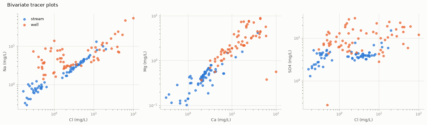
Sodium against chloride is close to a straight line over two orders of magnitude, which says a single dominant salinity source — road salt, here — diluted to varying degrees. Calcium against magnesium is a separate, tighter trend, which says rock weathering. Two processes, two directions, and the dilute end of both trends is the same weakly mineralised rainwater-derived water.

That paragraph is a conceptual model: a written statement of which source waters you believe exist and why, arrived at from hydrology and geology rather than from the numbers. It must come first, and no amount of computation substitutes for it. What the next notebook adds is a test — does the data actually require the number of sources you just proposed? — and after that, the proportions.

Note the log axes above, used only to see a wide range on one figure. Never feed log-transformed concentrations to a mixing calculation. Mixing is a weighted average of concentrations; the log of a weighted average is not the weighted average of the logs, so the transform breaks the one relationship the whole method depends on.

Use this in your own code

import pandas as pd
import mescla as am

samples = am.WaterChemistry.from_frame(pd.read_csv("samples.csv", index_col=0))

# 1. Screen before you model.
report = am.charge_balance_report(samples, tolerance=5.0)
clean = samples.select_rows([s for s, ok in zip(samples.samples, report["pass"]) if ok])

# 2. Convert when you need charge or stoichiometry.
meq = am.to_meq_per_l(clean)

# 3. Drop what you cannot defend, and say why in your notes.
usable = clean.drop_species(["NO3"])     # redox-active in this aquifer

Next: 02_emma_rank_and_endmembers.ipynb — counting the sources.

The classical diagrams

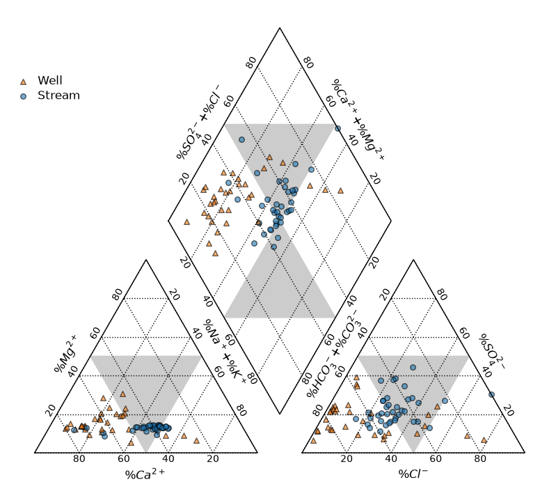
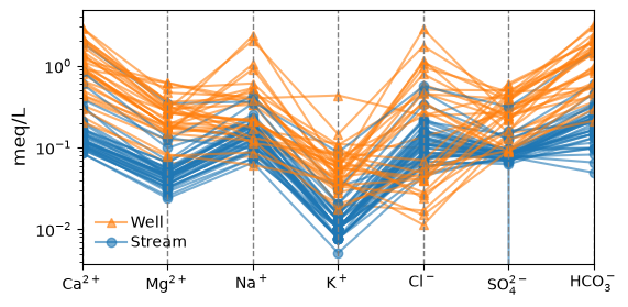
Bivariate plots are useful to the analyst. Piper, Schoeller, Stiff and the rest are what you put in front of everyone else — and mescla does not draw them. They are a solved problem: WQChartPy covers Piper (triangle, rectangle, coloured and contoured), Schoeller, Stiff, Durov, Chadha, Gibbs, Gaillardet and more, and takes a plain DataFrame:

pip install wqchartpy

The bundled Grafton dataset has no bicarbonate (its Water Quality Portal query never asked for it), and without one anion the ternaries collapse onto an edge instead of filling the triangle. Rather than fake it with HCO3=0.0, fetch the real bicarbonate for the same sites and dates and keep only the samples that have it:

import pandas as pd
from wqchartpy import triangle_piper, schoeller
from mescla.datasets import fetch_water_quality_portal, load_grafton_nh_frame

grafton = load_grafton_nh_frame()
bicarbonate = fetch_water_quality_portal(
    characteristics=("Bicarbonate",), siteid=tuple(grafton["site"].unique()),
)
bicarbonate["date"] = pd.to_datetime(bicarbonate["date"])
frame = grafton.merge(bicarbonate, on=["site", "date"]).rename(columns={"Bicarbonate": "HCO3"})

# WQChartPy wants Sample/Label/Color/Marker/Size/Alpha plus the major ions.
# Color and Marker are per-sample, so give Stream and Well distinct ones.
colors = frame["site_type"].map({"Stream": "tab:blue", "Well": "tab:orange"})
markers = frame["site_type"].map({"Stream": "o", "Well": "^"})
df = frame.assign(Sample=frame.index, Label=frame["site_type"],
                  Color=colors, Marker=markers, Size=30, Alpha=0.6, CO3=0.0)
triangle_piper.plot(df, unit="mg/L", figname="piper", figformat="png")
schoeller.plot(df, unit="mg/L", figname="schoeller", figformat="png")

Only 71 of the 130 samples (38 stream, 33 well) have a matching bicarbonate measurement, so the merge trims the dataset — a smaller diagram with real anions beats a full one with an invented edge case. CO3=0.0 stays because carbonate was never queried either — it is negligible next to bicarbonate at the near-neutral pH typical of these waters, but that is an assumption, not a measurement.

import pandas as pd
from wqchartpy import triangle_piper, schoeller
from mescla.datasets import fetch_water_quality_portal, load_grafton_nh_frame

grafton = load_grafton_nh_frame()
bicarbonate = fetch_water_quality_portal(
    characteristics=("Bicarbonate",), siteid=tuple(grafton["site"].unique()),
)
bicarbonate["date"] = pd.to_datetime(bicarbonate["date"])
frame = grafton.merge(bicarbonate, on=["site", "date"]).rename(columns={"Bicarbonate": "HCO3"})

# WQChartPy wants Sample/Label/Color/Marker/Size/Alpha plus the major ions.
# Color and Marker are per-sample, so give Stream and Well distinct ones.
colors = frame["site_type"].map({"Stream": "tab:blue", "Well": "tab:orange"})
markers = frame["site_type"].map({"Stream": "o", "Well": "^"})
df = frame.assign(Sample=frame.index, Label=frame["site_type"],
                  Color=colors, Marker=markers, Size=30, Alpha=0.6, CO3=0.0)
triangle_piper.plot(df, unit="mg/L", figname="piper", figformat="png")
schoeller.plot(df, unit="mg/L", figname="schoeller", figformat="png")

Trilinear Piper plot created. Saving it to /home/runner/work/mescla/mescla/docs/tutorials 

/opt/hostedtoolcache/Python/3.14.7/x64/lib/python3.14/site-packages/wqchartpy/schoeller.py:119: UserWarning: Attempt to set non-positive ylim on a log-scaled axis will be ignored.
  ax.set_ylim([np.min(meqL) * 0.5, np.max(meqL) * 1.5])

Schoeller diagram created. Saving it to /home/runner/work/mescla/mescla/docs/tutorials