06 · Reading reactions out of the residuals

A mixing model is a null hypothesis: this water is nothing but a blend of those waters. Where it fails, the failure is informative. Species that systematically depart from the mixing prediction are not measurement noise; they are the record of what happened to the water between its sources and your sampling point.

The convention:

	meaning	processes
measured > predicted	the system gained the species	dissolution, desorption, cation-exchange release, mineralisation
measured < predicted	the system lost it	precipitation, sorption, redox consumption, degradation, exchange uptake

This is half the value of doing mixing analysis at all, and it is how Tubau et al. (2014) identified carbonate dissolution, redox processes and ion exchange in the Besòs Delta.

import matplotlib.pyplot as plt
import numpy as np
import pandas as pd

import mescla as am
from mescla.datasets import make_mixture
from mescla.plotting import plot_measured_vs_predicted
from mescla.reactions.residuals import (
    classify_source_sink, fit_conservative, measured_vs_predicted, reaction_report,
)

A controlled experiment

We build a water that really is a three-source mixture, then make two things happen to it: calcium is added (30% more than mixing accounts for — carbonate dissolution) and sulphate is removed (30% less — sulphate reduction). Everything else stays conservative.

Because we did it ourselves, we know exactly what the method should find.

species = ["Cl", "Na", "Ca", "SO4", "Mg", "K"]
data = make_mixture(n_endmembers=3, n_species=6, n_samples=50,
                    endmember_noise=0.02, sample_noise=0.01, seed=11)
endmembers = am.EndMembers(data.true_endmembers.data, species, ("rain", "sea", "deep"))

altered = data.true_samples.copy()
altered[:, species.index("Ca")] *= 1.30     # gained:  dissolution
altered[:, species.index("SO4")] *= 0.70    # lost:    reduction
samples = am.WaterChemistry(altered, species, sigma=data.samples.sigma)

The trap: fitting with the reacting species

The obvious thing is to fit the ratios using everything you measured. Do not.

If a reacting species influences the ratios, least squares absorbs part of the reaction by shifting the ratios, and the residual is then smeared across every species. The reacting species looks nearly conservative, and innocent ones are convicted in its place.

naive = am.mixing_ratios(endmembers, samples)
naive_table = classify_source_sink(naive, samples)

print(f"ratios displaced from the truth by {np.abs(naive.ratios - data.true_ratios).mean():.3f} on average\n")
naive_table[["relative_departure", "behaviour"]].round(3)

ratios displaced from the truth by 0.069 on average

	relative_departure	behaviour
species
Cl	0.155	source
Na	-0.038	conservative
Ca	0.205	source
SO4	-0.215	sink
Mg	0.103	source
K	-0.042	conservative

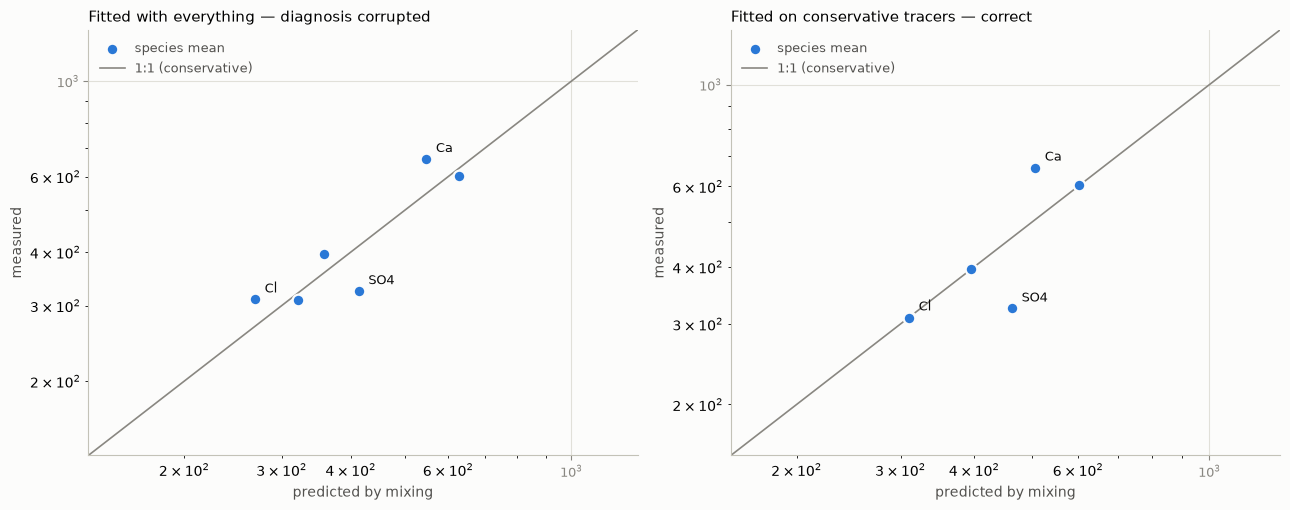
Look at what that produced. Calcium — enriched by a real 30% — is reported as conservative. Meanwhile species that we never touched are flagged as sinks. Every number is plausible and the diagnosis is wrong.

The fix: fit on the conservative tracers

Determine the ratios from the species you trust, then judge everything else against the mixture those ratios predict. Non-conservative species are not dropped — they are given a much larger standard deviation, so they contribute nothing to the fit but still receive a prediction to be compared against. This is precisely the device Tubau et al. used.

careful = fit_conservative(endmembers, samples, conservative=["Cl", "Na", "Mg", "K"])

print(f"ratios displaced from the truth by {np.abs(careful.ratios - data.true_ratios).mean():.4f} on average\n")
classify_source_sink(careful, samples)[
    ["mean_measured", "mean_predicted", "relative_departure", "behaviour", "likely_process"]
].round(3)

ratios displaced from the truth by 0.0000 on average

	mean_measured	mean_predicted	relative_departure	behaviour	likely_process
species
Cl	310.009	310.009	0.0	conservative
Na	309.475	309.475	-0.0	conservative
Ca	659.168	507.052	0.3	source	carbonate or gypsum dissolution; cation exchan...
SO4	324.210	463.157	-0.3	sink	sulphate reduction; gypsum precipitation
Mg	394.902	394.902	0.0	conservative
K	602.328	602.328	-0.0	conservative

The ratios are recovered essentially exactly, calcium is identified as a source at +30%, sulphate as a sink at −30%, and the four conservative tracers are left alone. Both magnitudes are right, because the departure is normalised by the prediction: “30% more calcium than conservative mixing accounts for”.

This is the single most important methodological point in the notebook. Fit on conservative tracers; judge the rest.

print(reaction_report(careful, samples))

Reaction screening based on constrained least squares (50 samples, 6 species)

Consistent with conservative mixing (4): Cl, Na, Mg, K

Gained relative to the mixing prediction (1):
  Ca       + 30.0% -- carbonate or gypsum dissolution; cation exchange release

Lost relative to the mixing prediction (1):
  SO4       -30.0% -- sulphate reduction; gypsum precipitation

These are hypotheses, not findings. Confirm with saturation indices (PHREEQC), redox measurements and a mineralogy that can supply or take up the species involved.

Note the hedging in the last line, and keep it. A departure from a mixing line is evidence consistent with a process. Confirming one needs saturation indices (PHREEQC), redox measurements, and a mineralogy that can actually supply or take up the species involved.

The figure

Points on the 1:1 line behave conservatively. Above it, the system gained the species; below, it lost it.

fig, axes = plt.subplots(1, 2, figsize=(13, 5.2))
plot_measured_vs_predicted(naive, samples, ax=axes[0], annotate=3)
axes[0].set_title("Fitted with everything — diagnosis corrupted", loc="left", fontsize=11)
plot_measured_vs_predicted(careful, samples, ax=axes[1], annotate=3)
axes[1].set_title("Fitted on conservative tracers — correct", loc="left", fontsize=11)
fig.tight_layout()

The one-panel summary

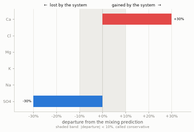
reaction_report gives you prose. This gives you the figure: sources one way, sinks the other, conservative species inside the shaded band. Polarity is the entire content, so it is drawn with a diverging pair and a neutral middle rather than with categorical colours.

from mescla.plotting import plot_reaction_departures

plot_reaction_departures(classify_source_sink(careful, samples), threshold=0.10);

How hard can it push before you notice?

Sensitivity of the screening to the size of the departure, at a fixed 10% threshold.

rows = []
for factor in [1.02, 1.05, 1.10, 1.20, 1.50, 2.00]:
    probe = data.true_samples.copy()
    probe[:, species.index("Ca")] *= factor
    chem = am.WaterChemistry(probe, species, sigma=data.samples.sigma)
    fit = fit_conservative(endmembers, chem, ["Cl", "Na", "Mg", "K"])
    table = classify_source_sink(fit, chem)
    rows.append({
        "Ca multiplied by": factor,
        "relative departure": round(float(table.loc["Ca", "relative_departure"]), 3),
        "p-value": f"{table.loc['Ca', 'p_value']:.1e}",
        "called": table.loc["Ca", "behaviour"],
    })
pd.DataFrame(rows).set_index("Ca multiplied by")

	relative departure	p-value	called
Ca multiplied by
1.02	0.02	8.4e-27	conservative
1.05	0.05	8.4e-27	conservative
1.10	0.10	8.4e-27	conservative
1.20	0.20	8.4e-27	source
1.50	0.50	8.4e-27	source
2.00	1.00	8.4e-27	source

With 50 clean samples, departures are detected statistically from about 2%, but the default 10% threshold deliberately withholds the verdict until the effect is chemically meaningful.

That threshold exists because statistical significance is not chemical significance: with enough samples a 1% departure becomes highly significant while remaining well inside analytical and conceptual error. Set it from what your laboratory and conceptual model can actually resolve, and say what you set it to.

The Besòs interpretation, for reference

Tubau et al. (2014) applied exactly this reasoning to the Besòs Delta aquifer in Barcelona and reported:

• Gained relative to the river mixing line: Mg and Ca (carbonate dissolution), plus Br, F, As, Fe and B (water–rock interaction, reductive desorption).

• Lost: O₂, NO₃ and TOC (redox processes) and K (exchanged for Ca or Mg on clays).

Note the internal consistency of that story — the same redox condition that consumes O₂ and NO₃ also consumes TOC and releases Fe and As by reductive dissolution of iron oxides. A reaction interpretation should hang together like that. A list of unrelated sources and sinks usually means the mixing model is wrong, not that the aquifer is strange.

Use this in your own code

from mescla.reactions.residuals import fit_conservative, classify_source_sink, reaction_report

# 1. Fit the ratios on the tracers you trust IN THIS SYSTEM.
result = fit_conservative(endmembers, samples, conservative=["Cl", "Br", "d18O"])

# 2. Judge every species against that fit.
table = classify_source_sink(result, samples, threshold=0.10)
table[table.behaviour != "conservative"]

# 3. A paragraph for your notes.
print(reaction_report(result, samples))

# 4. Then go and confirm it: saturation indices, redox data, a plausible mineralogy.

Next: 07_case_study_end_to_end.ipynb.