08 · Isotope tracers, and the one that breaks linear mixing¶

Isotopes are the workhorse tracers of recharge and hydrograph studies. They also contain the sharpest trap in the whole subject, because two kinds of isotope tracer behave completely differently and look identical in a spreadsheet.

	mixes linearly?	needs
δ¹⁸O, δ²H of the water molecule	yes	nothing
δ¹³C-DIC, δ³⁴S-SO₄, ⁸⁷Sr/⁸⁶Sr, δ¹⁵N-NO₃	no	weighting by the carrier element

Water isotopes are fine because water is the solvent: its “concentration” is the same in every end-member, so the weights in the mixing equation are just the mixing ratios.

A solute isotope ratio is carried by an element whose concentration differs between end-members, so the mixture is a concentration-weighted average:

\[\delta_{mix} = \frac{\sum_e f_e\, C_e\, \delta_e}{\sum_e f_e\, C_e}\]

which is nonlinear in \(f\). Feed such a tracer to an ordinary mixing calculation and you get a confident, plausible, wrong answer.

import matplotlib.pyplot as plt
import numpy as np
import pandas as pd

import mescla as am
from mescla.isotopes import (
    carrier_for, check_isotopes, delinearize, is_water_isotope,
    linearize, mix_isotope, two_component_isotope,
)
from mescla.mixing.geometric import two_component
from mescla.plotting.theme import LIGHT, apply_axes_style

How wrong, exactly?¶

Two end-members: dilute recharge with light carbon and little of it, and a deep water rich in heavy carbon. A 20-fold contrast in DIC — unremarkable in a real aquifer.

delta_1, carrier_1 = -24.0, 12.0     # recharge: d13C = -24 permil, DIC = 12 mg/L
delta_2, carrier_2 = -2.0, 250.0     # deep:     d13C =  -2 permil, DIC = 250 mg/L

fractions = np.linspace(0.0, 1.0, 21)
observed = np.array([
    float(mix_isotope(np.array([f, 1 - f]), np.array([delta_1, delta_2]),
                      np.array([carrier_1, carrier_2]))[0])
    for f in fractions
])

comparison = pd.DataFrame({
    "true f1": fractions,
    "delta observed": observed.round(2),
    "carrier-weighted": [two_component_isotope(d, delta_1, carrier_1, delta_2, carrier_2)
                         for d in observed],
    "naive formula": [two_component(d, delta_1, delta_2) for d in observed],
}).round(3)
comparison.iloc[::4]

	true f1	delta observed	carrier-weighted	naive formula
0	0.0	-2.00	0.0	-0.000
4	0.2	-2.26	0.2	0.012
8	0.4	-2.68	0.4	0.031
12	0.6	-3.48	0.6	0.067
16	0.8	-5.54	0.8	0.161
20	1.0	-24.00	1.0	1.000

Read the last two columns against the first. The carrier-weighted formula is exact. The naive one says 0.13 when the truth is 0.75 — the recharge contribution under-reported by a factor of six.

This is not a subtlety to note in the discussion section. It is the difference between “recharge dominates” and “recharge is negligible”.

fig, ax = plt.subplots(figsize=(6.8, 5.0))
ax.plot([0, 1], [0, 1], color=LIGHT.ink_muted, linewidth=1.2, zorder=1, label="truth")
ax.plot(fractions, comparison["carrier-weighted"], marker="o", markersize=6, linewidth=2,
        color=LIGHT.series[0], markeredgecolor=LIGHT.surface, markeredgewidth=1.4,
        zorder=3, label="carrier-weighted (correct)")
ax.plot(fractions, comparison["naive formula"], marker="s", markersize=6, linewidth=2,
        color=LIGHT.series[1], markeredgecolor=LIGHT.surface, markeredgewidth=1.4,
        zorder=2, label="naive delta formula")
ax.set_xlabel("true fraction of the recharge end-member")
ax.set_ylabel("estimated fraction")
ax.set_title("A solute isotope treated as an ordinary tracer", loc="left", fontsize=11)
apply_axes_style(ax, LIGHT)
ax.legend(frameon=False, fontsize=9)
fig.tight_layout()

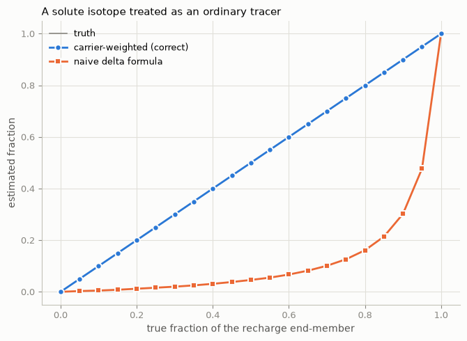
../_images/8fec9cd579d600fa53d8263b49c3b92b07af602d5914a9944ac7a44bba047bae.png

The curvature is the carrier weighting. The two agree only where the end-members share a carrier concentration, which is the special case the naive formula silently assumes.

The fix, and why it composes with everything else¶

The numerator of the weighted average is linear in \(f\), and so is the carrier concentration. So while \(\delta\) does not mix linearly, the product \(\delta \times C\) does:

\[(\delta C)_{mix} = \sum_e f_e\, (\delta C)_e\]

linearize() replaces each solute-isotope column with that product. After it, every estimator, diagnostic and plot in Mescla works unchanged — the fix is a transform, not a special case threaded through the library.

species = ("Cl", "SO4", "DIC", "d13C")
compositions = np.array([
    [  5.0,   3.0,  12.0, -24.0],    # rain: DIC-poor, light carbon
    [400.0, 120.0, 250.0,  -2.0],    # deep: DIC-rich, heavy carbon
    [ 80.0,  60.0,  60.0, -14.0],    # soil
])
endmembers = am.EndMembers(compositions, species, ("rain", "deep", "soil"))

# Build a truthful mixture: conservative species mix linearly, d13C does not.
true_ratios = np.random.default_rng(0).dirichlet(np.ones(3), 80)
values = np.empty((80, 4))
values[:, :3] = true_ratios @ compositions[:, :3]
values[:, 3] = mix_isotope(true_ratios, compositions[:, 3], compositions[:, 2])
samples = am.WaterChemistry(values, species)

samples.to_frame().describe().round(2)

	Cl	SO4	DIC	d13C
count	80.00	80.00	80.00	80.00
mean	166.86	61.58	110.39	-6.17
std	85.60	23.11	51.32	3.50
min	36.91	15.35	32.11	-15.11
25%	87.44	44.08	63.00	-7.73
50%	154.05	59.09	102.74	-4.81
75%	237.06	76.25	153.08	-3.44
max	369.88	113.16	232.02	-2.22

# The property everything rests on: the product is linear in the mixing ratios.
linear_endmembers = linearize(endmembers)
linear_samples = linearize(samples)

print("delta * C mixes linearly:",
      np.allclose(true_ratios @ linear_endmembers.data, linear_samples.data))
# Only the isotope column is relabelled; the others keep their own unit.
print("units after linearising:", linear_endmembers.units_dict())

delta * C mixes linearly: True
units after linearising: {'Cl': 'mg/L', 'SO4': 'mg/L', 'DIC': 'mg/L', 'd13C': 'linearised (mg/L x mg/L)'}

import warnings

with warnings.catch_warnings():
    warnings.simplefilter("ignore")
    naive = am.mixing_ratios(endmembers, samples)
correct = am.mixing_ratios(linear_endmembers, linear_samples)

for label, result in [("d13C used raw", naive), ("d13C linearised", correct)]:
    error = np.abs(result.ratios - true_ratios)
    print(f"  {label:20s} mean error {error.mean():.4f}   max error {error.max():.4f}")

  d13C used raw        mean error 0.0216   max error 0.0589
  d13C linearised      mean error 0.0000   max error 0.0000

Exact recovery once linearised. Note that the error in the raw case (about 0.02 on average) is smaller here than in the two-component example — because three conservative species are also present and partly compensate. That is the dangerous case: the bias is small enough to look like noise and large enough to change a conclusion.

The library will not let this pass silently¶

with warnings.catch_warnings(record=True) as caught:
    warnings.simplefilter("always")
    am.mixing_ratios(endmembers, samples)
    print(caught[0].message)

'd13C' is an isotope ratio of a solute, so it does NOT mix linearly: it must be weighted by its carrier (DIC or HCO3 or TIC or alkalinity). Using it as an ordinary tracer gives wrong mixing ratios. Fix with: linearize(table, {'d13C': 'DIC'})

A warning rather than an error: you might have a reason, and refusing would be presumptuous. Silence would not be.

check_isotopes is the same check, callable directly:

print("before:", check_isotopes(samples))
print("after: ", check_isotopes(linear_samples))

before: ["'d13C' is an isotope ratio of a solute, so it does NOT mix linearly: it must be weighted by its carrier (DIC or HCO3 or TIC or alkalinity). Using it as an ordinary tracer gives wrong mixing ratios. Fix with: linearize(table, {'d13C': 'DIC'})"]
after:  []

Which labels are recognised¶

Matching ignores formatting and handles the compound forms used in the literature. The distinction that matters most is oxygen: δ¹⁸O alone is the water molecule; δ¹⁸O-NO₃ and δ¹⁸O-SO₄ are not.

labels = ["d18O", "d2H", "δ18O", "d13C", "d13C-DIC", "d34S", "δ34S−SO4",
          "87Sr/86Sr", "d15N-NO3", "d18O-NO3", "Cl", "SO4-S"]
pd.DataFrame({
    "label": labels,
    "water isotope (mixes linearly)": [is_water_isotope(name) for name in labels],
    "carrier required": [carrier_for(name) for name in labels],
}).set_index("label")

	water isotope (mixes linearly)	carrier required
label
d18O	True	None
d2H	True	None
δ18O	True	None
d13C	False	(DIC, HCO3, TIC, alkalinity)
d13C-DIC	False	(DIC, HCO3, TIC, alkalinity)
d34S	False	(SO4,)
δ34S−SO4	False	(SO4,)
87Sr/86Sr	False	(Sr,)
d15N-NO3	False	(NO3,)
d18O-NO3	False	(NO3,)
Cl	False	None
SO4-S	False	None

Reporting predictions back in delta units¶

After linearisation the fitted values are in \(\delta \times C\) units, which no one wants to read. delinearize converts them back.

carrier_column = samples.data[:, samples.species.index("DIC")]
predicted_delta = delinearize(correct.fitted[:, species.index("d13C")], carrier_column)

pd.DataFrame({
    "measured d13C": samples.data[:, 3][:6].round(2),
    "predicted d13C": predicted_delta[:6].round(2),
}, index=samples.samples[:6])

	measured d13C	predicted d13C
sample1	-2.73	-2.73
sample2	-6.99	-6.99
sample3	-8.03	-8.03
sample4	-3.79	-3.79
sample5	-14.50	-14.50
sample6	-2.58	-2.58

Water isotopes need none of this¶

sea = am.EndMembers([[5.0, -12.0], [400.0, -4.0]],
                    species=["Cl", "d18O"], index=["rain", "seawater"])
weights = np.linspace(0.05, 0.95, 20)[:, None]
weights = np.hstack([weights, 1 - weights])
brackish = am.WaterChemistry(weights @ sea.data, ("Cl", "d18O"))

result = am.mixing_ratios(sea, brackish)
print("d18O used directly, max error:", np.abs(result.ratios - weights).max())
print("no warning issued:", check_isotopes(brackish) == [])

d18O used directly, max error: 1.27675647831893e-14
no warning issued: True

Use this in your own code¶

import mescla as am
from mescla.isotopes import linearize, delinearize, check_isotopes

# 1. Ask the library what needs treatment. It also warns you automatically.
print(check_isotopes(samples))

# 2. Linearise BOTH tables -- the same transform, like standardisation.
#    Carriers are inferred from the labels; pass them explicitly if you prefer.
linear_samples = linearize(samples, {"d13C": "DIC", "d34S": "SO4"})
linear_endmembers = linearize(endmembers, {"d13C": "DIC", "d34S": "SO4"})

# 3. Everything downstream is unchanged.
model = am.EMMA().fit(linear_samples)
result = am.mixing_ratios(linear_endmembers, linear_samples)

# 4. Convert predictions back for reporting.
carrier = samples.data[:, samples.species.index("DIC")]
predicted = delinearize(result.fitted[:, samples.species.index("d13C")], carrier)

# Two components and one isotope? There is a closed form:
from mescla.isotopes import two_component_isotope
f1 = two_component_isotope(delta_sample, delta_1, DIC_1, delta_2, DIC_2)

A caveat worth keeping. Linearisation makes the mixing correct. It does not make the isotope conservative: δ¹³C is altered by carbonate dissolution, degassing and methanogenesis, and δ³⁴S by sulphate reduction. Treat a linearised isotope like any other tracer whose conservativeness you must argue for — notebook 06 shows how to test it rather than assume it.