05 · Uncertainty and identifiability

Never report a mixing fraction without an uncertainty. A mixing ratio is an estimate from noisy inputs through a constrained inverse problem; quoted bare, it claims a precision it does not have.

Four routes, in rising order of effort, plus the diagnostics that tell you whether the problem was answerable in the first place.

import matplotlib.pyplot as plt
import numpy as np
import pandas as pd

import mescla as am
from mescla.datasets import make_mixture
from mescla.plotting.theme import LIGHT, apply_axes_style
from mescla.uncertainty.identifiability import (
    condition_number, endmember_separation, identifiability_report, sigma_sweep,
)
from mescla.uncertainty.montecarlo import monte_carlo_ratios
from mescla.uncertainty.propagation import genereux_sigma
from mescla.uncertainty.resampling import bootstrap_endmembers, jackknife_endmembers

1. Gaussian propagation (Genereux, 1998)

The standard for two-component separations. With \(f_1 = (C_s - C_2)/(C_1 - C_2)\):

\[\sigma_{f_1}^2 = \left[\frac{C_s - C_2}{(C_1-C_2)^2}\sigma_{C_1}\right]^2 + \left[\frac{C_s - C_1}{(C_1-C_2)^2}\sigma_{C_2}\right]^2 + \left[\frac{\sigma_{C_s}}{C_1-C_2}\right]^2\]

The lesson is in the denominator: uncertainty scales as \(1/(C_1-C_2)\).

contrasts = [10, 20, 50, 100, 200, 500]
sigmas = [genereux_sigma(c / 2, c_1=c, c_2=0.0, sd_sample=1.0, sd_1=3.0, sd_2=3.0)
          for c in contrasts]

fig, ax = plt.subplots(figsize=(6.6, 4.2))
ax.plot(contrasts, sigmas, marker="o", markersize=7, linewidth=2, color=LIGHT.series[0],
        markeredgecolor=LIGHT.surface, markeredgewidth=1.6)
ax.set_xscale("log"); ax.set_yscale("log")
ax.set_xlabel("end-member contrast  $C_1 - C_2$  (mg/L)")
ax.set_ylabel(r"$\sigma$ of the mixing fraction")
ax.set_title("Contrast buys precision that the laboratory cannot", loc="left", fontsize=11)
apply_axes_style(ax, LIGHT)

pd.DataFrame({"contrast": contrasts, "sigma_f": np.round(sigmas, 4)}).set_index("contrast")

	sigma_f
contrast
10	0.2345
20	0.1173
50	0.0469
100	0.0235
200	0.0117
500	0.0047

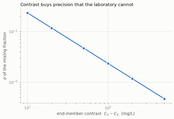
A tracer separating the end-members by 10 mg/L gives ±0.23 on the fraction — useless. At 500 mg/L it gives ±0.005. Choosing tracers with wide contrast matters more than measuring them precisely, and no amount of analytical care compensates for a poor choice.

One warning: feed these formulas the standard deviation that reflects the spatial and temporal variability of the end-member, not the laboratory’s repeatability. The latter is typically an order of magnitude too optimistic and produces indefensible intervals.

print("if you use the lab's precision (0.5 mg/L):       ",
      round(genereux_sigma(50.0, 100.0, 0.0, 1.0, 0.5, 0.5), 4))
print("if you use the real end-member variability (15):",
      round(genereux_sigma(50.0, 100.0, 0.0, 1.0, 15.0, 15.0), 4))

if you use the lab's precision (0.5 mg/L):        0.0106
if you use the real end-member variability (15): 0.1065

A factor of eight in the reported uncertainty, from one honest choice.

2. Monte Carlo

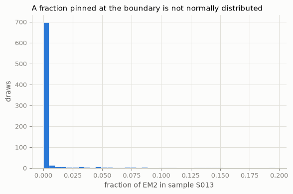
Analytical propagation assumes local linearity and ignores the simplex constraints. Monte Carlo does neither: it re-solves the constrained problem for every draw, so the intervals respect closure and non-negativity by construction. That matters most exactly where it is needed — near the edge of the mixing hull, where a fraction is pinned at zero and the sampling distribution is strongly asymmetric.

data = make_mixture(n_endmembers=3, n_species=5, n_samples=25, seed=4)
mc = monte_carlo_ratios(data.endmembers, data.samples, n_draws=800, seed=0)

summary = pd.DataFrame({
    "estimate": mc["mean"][:, 0].round(3),
    "sd": mc["sd"][:, 0].round(3),
    "2.5%": mc["lower"][:, 0].round(3),
    "97.5%": mc["upper"][:, 0].round(3),
    "true": data.true_ratios[:, 0].round(3),
}, index=data.samples.samples)
summary.head(8)

	estimate	sd	2.5%	97.5%	true
S001	0.477	0.072	0.345	0.624	0.380
S002	0.170	0.074	0.009	0.312	0.070
S003	0.904	0.076	0.734	1.000	0.828
S004	0.451	0.068	0.310	0.582	0.344
S005	0.809	0.088	0.638	1.000	0.715
S006	0.148	0.078	0.000	0.302	0.061
S007	0.156	0.076	0.000	0.293	0.058
S008	0.348	0.066	0.212	0.480	0.227

covered = ((data.true_ratios >= mc["lower"]) & (data.true_ratios <= mc["upper"])).mean()
print(f"fraction of true ratios inside the 95% interval: {covered:.1%}")

fraction of true ratios inside the 95% interval: 93.3%

Near-nominal coverage — the intervals are honest rather than decorative.

Skewness near the boundary, which is exactly what analytical propagation would miss:

edge = int(np.argmin(mc["mean"].min(axis=1)))
draws = mc["draws"][:, edge, :]
pinned = int(np.argmin(mc["mean"][edge]))

fig, ax = plt.subplots(figsize=(6.6, 4.0))
ax.hist(draws[:, pinned], bins=40, color=LIGHT.series[0], edgecolor=LIGHT.surface, linewidth=0.5)
ax.set_xlabel(f"fraction of {data.endmembers.labels[pinned]} in sample {data.samples.samples[edge]}")
ax.set_ylabel("draws")
ax.set_title("A fraction pinned at the boundary is not normally distributed",
             loc="left", fontsize=11)
apply_axes_style(ax, LIGHT)
print(f"{(draws[:, pinned] <= 1e-9).mean():.0%} of draws sit exactly at zero")

86% of draws sit exactly at zero

Show the intervals, do not tabulate them

A stacked bar of point estimates cannot express that a fraction is ±0.1. This can, and it is the figure that stops a reader arguing about a five-point difference between two samples.

from mescla.plotting import plot_ratios_with_uncertainty

result = am.mixing_ratios(data.endmembers, data.samples)
plot_ratios_with_uncertainty(result, mc, order_by=0);

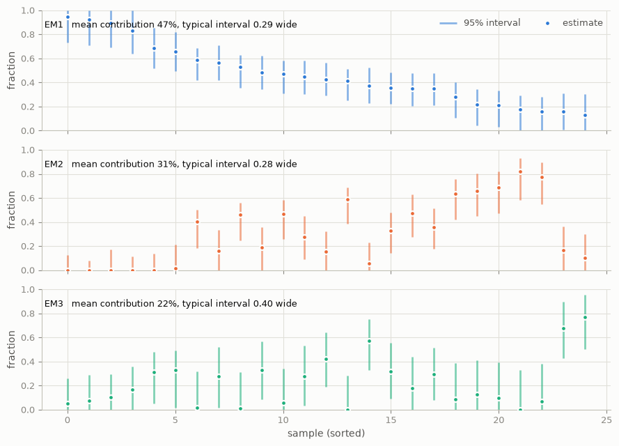
A symmetric ± interval around this would be nonsense. Use percentiles.

3. Resampling: measure the uncertainty instead of asserting it

Propagation and Monte Carlo need you to state the end-member uncertainty. Resampling measures it, from the replicate samples that define each end-member — usually the honest route, because the dominant error is how well a handful of samples represents a source water, not how well the laboratory measured them.

rng = np.random.default_rng(0)
centres = {
    "rainfall":   np.array([2.0, 1.0, 0.5, 8.0, 3.0]),
    "seawater":   np.array([19000.0, 10500.0, 400.0, 1290.0, 2700.0]),
    "deep brine": np.array([5000.0, 2000.0, 1500.0, 300.0, 40.0]),
}
# Six replicate analyses of each source, with realistic spread.
replicates = {name: rng.normal(v, 0.12 * v, size=(6, 5)) for name, v in centres.items()}

true_mix = rng.dirichlet([2, 2, 2], size=12)
observed = am.WaterChemistry(
    true_mix @ np.vstack(list(centres.values())),
    species=["Cl", "Na", "SO4", "HCO3", "Ca"],
)

jack = jackknife_endmembers(replicates, observed)
boot = bootstrap_endmembers(replicates, observed, n_draws=400)

pd.DataFrame({
    "estimate": jack["ratios"][:, 1].round(3),
    "jackknife sd": jack["sd"][:, 1].round(3),
    "bootstrap 2.5%": boot["lower"][:, 1].round(3),
    "bootstrap 97.5%": boot["upper"][:, 1].round(3),
    "true": true_mix[:, 1].round(3),
}).head(8)

	estimate	jackknife sd	bootstrap 2.5%	bootstrap 97.5%	true
0	0.265	0.013	0.241	0.284	0.260
1	0.107	0.007	0.096	0.118	0.098
2	0.560	0.025	0.512	0.593	0.564
3	0.383	0.017	0.363	0.409	0.377
4	0.426	0.020	0.389	0.453	0.426
5	0.287	0.013	0.262	0.306	0.286
6	0.491	0.023	0.450	0.521	0.491
7	0.213	0.011	0.194	0.230	0.205

Use the jackknife for a quick symmetric standard deviation, and the bootstrap when a fraction sits near zero and its distribution is skewed.

4. Identifiability: was the question answerable at all?

Three failure modes recur, and all three produce confident-looking numbers rather than errors: uncertain end-member definition, poor tracer choice, and colinearity.

Here is colinearity, constructed deliberately: two end-members that are nearly the same water.

distinct = am.EndMembers([[10.0, 500.0], [900.0, 20.0], [400.0, 400.0]],
                         species=["Cl", "SO4"], index=["A", "B", "C"])
collinear = am.EndMembers([[10.0, 500.0], [900.0, 20.0], [880.0, 35.0]],
                          species=["Cl", "SO4"], index=["A", "B", "B_lookalike"])

for name, em in [("distinct", distinct), ("nearly collinear", collinear)]:
    print(f"{name:18s} condition number = {condition_number(em):7.1f}")
    print(endmember_separation(em).round(3).to_string(index=False))
    print()

distinct           condition number =     1.4
 pair  distance  relative
A - C     1.175     0.349
B - C     2.294     0.681
A - B     3.370     1.000

nearly collinear   condition number =     1.4
           pair  distance  relative
B - B_lookalike     0.083     0.027
A - B_lookalike     2.958     0.973
          A - B     3.040     1.000

Rules of thumb: condition number below 10 is comfortable, above 30 a warning, above 100 means the ratios are not reliably identifiable. A relative separation below 0.2 means that pair is effectively one source — merge them or drop one.

identifiability_report runs every check and returns a verdict table. Run it before believing any result.

samples = am.WaterChemistry(
    np.random.default_rng(1).dirichlet([2, 2, 2], 30) @ distinct.data,
    species=["Cl", "SO4"],
)
identifiability_report(distinct, samples)

	value	verdict	note
check
condition number of end-member matrix	1.4	pass	colinear end-members make ratios unstable
closest end-member pair (A - C)	0.349	warn	relative separation; below 0.2 the pair is eff...
species available vs required	2 vs 2	warn	ne-1 species are the bare minimum; redundancy ...
samples outside the mixing hull (unconstrained solve)	0%	pass	most negative unconstrained ratio 0.035; a mis...

identifiability_report(collinear, samples)

	value	verdict	note
check
condition number of end-member matrix	1.4	pass	colinear end-members make ratios unstable
closest end-member pair (B - B_lookalike)	0.027	fail	relative separation; below 0.2 the pair is eff...
species available vs required	2 vs 2	warn	ne-1 species are the bare minimum; redundancy ...
samples outside the mixing hull (unconstrained solve)	100%	fail	most negative unconstrained ratio -18.244; a m...

5. The sigma sweep — always report it

Notebook 04 showed that assigning standard deviations changes the answer. That makes it a result to be shown, not a setting to be buried. sigma_sweep refits with the end-member sigmas scaled up and down; this is the MIX_1 / MIX_2 comparison in Tubau et al. (2014).

If the mean contributions move by more than a few percent across the sweep, the variance assumptions are doing the work, not your data.

data = make_mixture(n_endmembers=3, n_species=6, n_samples=40,
                    endmember_noise=0.15, sample_noise=0.02, seed=5)
sigma_sweep(data.endmembers, data.samples, factors=(0.1, 0.5, 1.0, 2.0, 10.0)).round(4)

	sigma_factor	mean_EM1	mean_EM2	mean_EM3	max_ratio_shift_vs_reference
0	0.1	0.3035	0.3325	0.3640	0.0000
1	0.5	0.2963	0.3223	0.3813	0.0498
2	1.0	0.2963	0.3214	0.3823	0.0000
3	2.0	0.2962	0.3270	0.3768	0.0116
4	10.0	0.3061	0.3332	0.3606	0.0381

Use this in your own code

from mescla.uncertainty.propagation import genereux_sigma
from mescla.uncertainty.montecarlo import monte_carlo_ratios
from mescla.uncertainty.resampling import jackknife_endmembers
from mescla.uncertainty.identifiability import identifiability_report, sigma_sweep

# 0. Before anything: is the problem answerable?
print(identifiability_report(endmembers, samples))

# 1. Two components, one tracer -- the quick analytical answer.
sd = genereux_sigma(c_sample, c_1, c_2, sd_sample, sd_1, sd_2)   # use VARIABILITY, not lab precision

# 2. Several components, or fractions near the boundary.
mc = monte_carlo_ratios(endmembers, samples, n_draws=2000)
lower, upper = mc["lower"], mc["upper"]

# 3. You have replicate analyses of each source -- measure it instead.
jack = jackknife_endmembers({"rain": rain_replicates, "river": river_replicates}, samples)

# 4. Report the sensitivity to your own assumptions.
sigma_sweep(endmembers, samples).to_csv("sigma_sensitivity.csv")

Next: 06_reactions_from_residuals.ipynb — what the misfit is telling you.