07 · A complete analysis, start to finish

Everything from the previous notebooks applied once, in order, to real data — written so you can copy the structure for your own study.

Question. What waters make up stream flow in Grafton County, New Hampshire, and in what proportions?

Data. 66 stream samples with six major ions (Ca, Mg, Na, K, Cl, SO₄), 1990–2021, from the USGS via the Water Quality Portal. Public domain; provenance in src/mescla/datasets/data/SOURCES.md.

The workflow, which is the same every time:

1. Conceptual model first — what could the sources be?

2. Characterise and screen the chemistry.

3. EMMA: how many end-members, which species.

4. Choose end-members and check they bound the data.

5. Compute mixing ratios.

6. Quantify uncertainty.

7. Read the residuals as chemistry.

8. State the conclusion and its limitations.

import matplotlib.pyplot as plt
import numpy as np
import pandas as pd

import mescla as am
from mescla.datasets import load_grafton_nh, load_grafton_nh_frame
from mescla.plotting import (
    plot_measured_vs_predicted, plot_mixing_line, plot_ratios, plot_scree, plot_uspace,
)
from mescla.reactions.residuals import classify_source_sink, fit_conservative
from mescla.uncertainty.montecarlo import monte_carlo_ratios

Step 1 — Conceptual model, before touching the data

New England upland streams in a glaciated, forested catchment with roads. Plausible sources:

• Precipitation / snowmelt — very dilute in everything.

• Weathering of till and bedrock — supplies Ca, Mg, SO₄, some K.

• Road salt — halite: Na and Cl together, in near-equal equivalents.

• Possibly septic or agricultural inputs, which we have no tracer for here.

That is three sources we can hope to resolve with six major ions, which means we should expect EMMA to want about k = 2. Writing the expectation down first is what makes the result a test rather than a rationalisation.

Step 2 — Restrict to one system, then screen

Notebook 02 fitted all 130 samples — streams and wells together — and every species came back poor. That was the right answer: those are not one mixing system. A well-posed EMMA needs samples from one system with stable end-members.

samples = load_grafton_nh("Stream")
frame = load_grafton_nh_frame("Stream")
print(samples)
samples.to_frame().describe().round(2)

<WaterChemistry: 66 rows x 6 species [mg/L, no sigma]
  species: Ca, Mg, Na, K, Cl, SO4>

	Ca	Mg	Na	K	Cl	SO4
count	66.00	66.00	66.00	66.00	66.00	66.00
mean	3.31	0.52	2.66	0.46	3.21	4.07
std	5.04	0.54	2.42	0.42	3.86	1.83
min	0.31	0.10	0.29	0.12	0.17	1.29
25%	1.54	0.31	0.83	0.30	0.36	3.38
50%	2.26	0.44	2.15	0.40	2.45	3.90
75%	3.00	0.56	3.62	0.50	4.55	4.39
max	38.00	4.20	13.10	3.40	20.00	15.00

Three orders of magnitude in chloride. That is the range we need — and its likely cause, road salt, is one of the sources we listed.

Known limitation, stated up front: the dataset has no bicarbonate, so charge balance cannot be checked properly (see notebook 01). In a study for publication you would go back for alkalinity before going further. We proceed knowingly.

report = am.charge_balance_report(samples)
print(f"charge balance passing: {report['pass'].sum()} of {len(report)} "
      f"(median CBE {report['cbe_percent'].median():+.0f}% — the missing HCO3)")

charge balance passing: 2 of 66 (median CBE +26% — the missing HCO3)

Step 3 — EMMA

model = am.EMMA().fit(samples)
print(model.summary())
print()
print("rank criteria:", model.rank_summary().attrs["recommendations"])

EMMA on 66 samples x 6 species (standardize=True, rule='one')
  retained k = 1 component(s), explaining 81.2% of the variance
  => 2 end-members required
  eigenvalues: [4.875 0.876 0.159 0.046 0.031 0.012]
  species fitting poorly: ['Ca', 'Mg', 'Na', 'K', 'Cl']

rank criteria: {'rule_of_one': 1, 'cumulative_variance': 2, 'broken_stick': 1, 'parallel_analysis': 1}

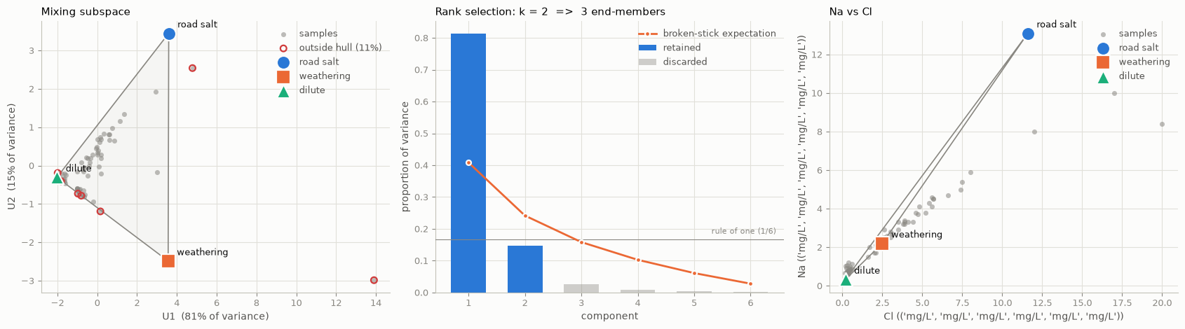
The criteria disagree — the rule of one, broken-stick and parallel analysis say k = 1, cumulative variance says k = 2. Rather than pick by rule, look at what the components mean and at how the fit improves:

rows = []
for k in [1, 2, 3]:
    trial = am.EMMA(k=k).fit(samples)
    diagnostics = trial.diagnostics().to_frame()
    rows.append({
        "k": k,
        "end-members": k + 1,
        "variance explained": round(float(trial.eigenvalues_[:k].sum() / trial.eigenvalues_.sum()), 3),
        "mean RRMSE": round(float(diagnostics["rrmse"].mean()), 3),
        "species fitting poorly": int((diagnostics["verdict"] == "poor").sum()),
    })
pd.DataFrame(rows).set_index("k")

	end-members	variance explained	mean RRMSE	species fitting poorly
k
1	2	0.812	0.409	5
2	3	0.959	0.176	1
3	4	0.985	0.124	0

Going from k = 1 to k = 2 takes the variance from 81% to 96% and the number of poorly fitting species from five to one. Going on to k = 3 buys much less. k = 2 ⟹ three end-members — which is what the conceptual model predicted.

model = am.EMMA(k=2).fit(samples)
model.loadings_frame().iloc[:, :3].round(3)

	EV1	EV2	EV3
Ca	0.417	-0.370	-0.165
Mg	0.438	-0.200	-0.315
Na	0.335	0.708	0.182
K	0.433	-0.246	-0.198
Cl	0.399	0.476	-0.303
SO4	0.419	-0.187	0.842

This is the moment the analysis becomes chemistry:

• EV1 — every species positive and roughly equal: the dilution axis. How much water versus how much solute.

• EV2 — Na (+0.71) and Cl (+0.48) against Ca (−0.37), K (−0.25), Mg (−0.20), SO₄ (−0.19): road salt against weathering.

Two axes, exactly the two processes we predicted, and the third source (dilute precipitation) is the origin they both radiate from.

model.diagnostics().to_frame().round(3)

	relative_bias	rrmse	verdict
Ca	0.0	0.265	poor
Mg	0.0	0.170	suspect
Na	0.0	0.110	suspect
K	-0.0	0.169	suspect
Cl	0.0	0.191	suspect
SO4	-0.0	0.151	suspect

Step 4 — Choose end-members and check they bound the data

End-members should be real measured waters, not centroids — that keeps them chemically self-consistent. We take the most extreme samples in U-space as candidates and ask which combination encloses the most samples.

distance = np.linalg.norm(model.scores_ - model.scores_.mean(axis=0), axis=1)
candidates = samples.select_rows([samples.index[i] for i in np.argsort(-distance)[:8]])

model.suggest_endmembers(candidates, n_endmembers=3).head(4).round(3)

	endmembers	fraction_enclosed	volume
0	S046, S010, S058	0.894	16.612
1	S010, S035, S058	0.773	11.656
2	S037, S010, S058	0.712	15.381
3	S046, S010, S065	0.697	16.504

chosen = samples.select_rows(
    model.suggest_endmembers(candidates, 3).iloc[0]["endmembers"].split(", ")
)
print(f"samples enclosed: {model.hull_fraction(chosen):.0%}\n")

labelled = frame.loc[[list(samples.index).index(name) for name in chosen.index],
                     ["site", "date"]].reset_index(drop=True)
display = chosen.to_frame().round(2).reset_index(drop=True)
pd.concat([labelled, display], axis=1)

samples enclosed: 89%

	site	date	Ca	Mg	Na	K	Cl	SO4
0	USGS-434509072073101	2010-10-28	4.30	0.58	13.10	0.75	11.60	7.79
1	USGS-01137500	1993-09-15	17.00	1.60	2.20	1.30	2.50	7.70
2	USGS-440825071431001	2011-05-22	0.42	0.11	0.33	0.29	0.18	1.29

Read them against the conceptual model:

	character	interpretation
first	Na 13.1, Cl 11.6, Ca 4.3	road salt — Na and Cl dominant
second	Ca 17.0, SO₄ 7.7, Na 2.2	weathering — Ca and SO₄ dominant
third	everything below 1.3 mg/L	dilute precipitation / snowmelt

Three real stream samples, each behaving as one of the three sources we hypothesised before looking. Let us name them accordingly.

endmembers = am.EndMembers(chosen.data, chosen.species, ("road salt", "weathering", "dilute"))

fig, axes = plt.subplots(1, 3, figsize=(17, 4.8))
plot_uspace(model, endmembers, ax=axes[0])
plot_scree(model, ax=axes[1])
plot_mixing_line(samples, endmembers, ("Cl", "Na"), ax=axes[2])
fig.tight_layout()

Would an algorithm have chosen the same three?

We picked those end-members by taking extreme samples in U-space and testing combinations — a hand-rolled vertex search. Archetypal analysis is the optimised form of the same step (notebook 02), and running it here is a test of Step 1 rather than a replacement for it: the conceptual model named road salt, weathering and dilute precipitation before the data were examined, and the algorithm has never heard of any of them.

arch = model.archetypes(seed=0)
print(arch.summary())

print(f"\nenclosed by our three:   {model.hull_fraction(endmembers):.0%}")
print(f"enclosed by archetypes:  {arch.hull_fraction:.0%}")

pd.concat(
    {"archetypes": arch.archetypes_frame().round(2),
     "chosen by hand": endmembers.to_frame().round(2)},
    axis=0,
)

Archetypal analysis: 3 archetypes on 66 samples x 6 species (space='uspace', seed=0)
  explained variance = 99.4% (RSS 2.065)
  restarts = 10, reaching the best objective = 100%
  converged = True in 9 iterations
  samples effectively supporting each archetype: [1.1 1.  1. ]
  fraction of samples enclosed = 0.64
  archetypes with negative concentrations: {'A1': ['Cl']}
  These are candidates, not end-members: name them against the conceptual model first.
  The weights are not mixing ratios -- pass .as_endmembers() to mixing_ratios() or mix_ml().

enclosed by our three:   89%
enclosed by archetypes:  64%

		Ca	Mg	Na	K	Cl	SO4
archetypes	A1	0.21	0.13	0.49	0.17	-0.34	2.81
	A2	38.09	4.12	8.79	3.32	19.08	15.69
	A3	4.43	1.00	11.47	0.76	15.07	5.63
chosen by hand	road salt	4.30	0.58	13.10	0.75	11.60	7.79
	weathering	17.00	1.60	2.20	1.30	2.50	7.70
	dilute	0.42	0.11	0.33	0.29	0.18	1.29

fig, axes = plt.subplots(1, 2, figsize=(13, 5), sharex=True, sharey=True)
plot_uspace(model, endmembers, ax=axes[0])
axes[0].set_title("Chosen by hand: maximise enclosure", loc="left")
plot_uspace(model, arch.as_endmembers(), ax=axes[1])
axes[1].set_title("Archetypes: minimise reconstruction error", loc="left")
fig.tight_layout()

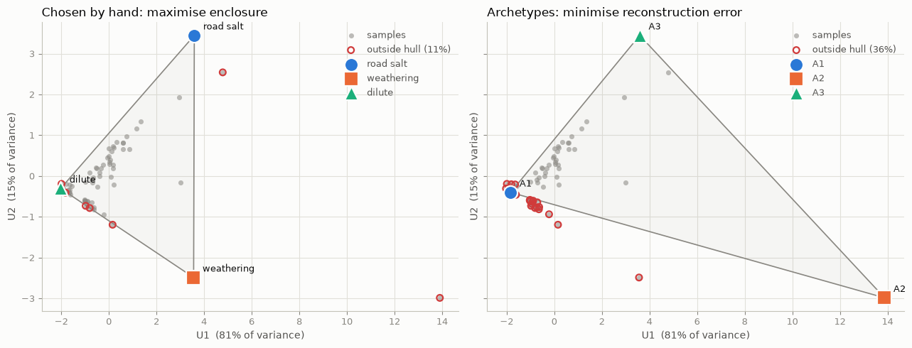
Two of the three vertices agree, and one does not.

The road-salt archetype is the same sample we picked by hand — identical U-space coordinates. Its concentrations in the table differ a little because an archetype is reported as its rank-2 reconstruction, not as the raw analysis. The dilute archetype is one sample away from ours and slightly less extreme. On those two, an unsupervised objective that knows nothing about New England, roads or till arrived at the conceptual model written down in Step 1, which is worth more as corroboration than any fit statistic in this notebook.

The third vertex is a different water entirely. Ours is a Ca–SO₄ weathering sample; the archetype is a heavily mineralised one with Ca 38 and Cl 19 mg/L, far out along the dilution axis. The figure shows the consequence: a long thin triangle that encloses 64% of the samples where ours encloses 89%.

That is not a bug, it is the two methods optimising different things. suggest_endmembers ranks vertex sets by how many samples they bound. Archetypal analysis minimises squared reconstruction error, and one extreme analysis contributes far more of that error than the sixty ordinary ones — so the optimiser spends a vertex on it. Whenever the two disagree this sharply, the useful move is to go and look at the sample the optimiser latched onto rather than to declare a winner. Here it is a single very concentrated stream analysis, which is worth a QA/QC look and is quite possibly one of the 11% this study cannot explain.

Three further reasons the hand-picked set stays.

1. One archetype returns a negative chloride, flagged in the summary above. It is a rank-2 reconstruction, not a water, and no negative concentration is a water. chosen are real analyses that can be defended sample by sample, with a site and a date.

2. n_effective is close to 1 for each archetype, so they rest on essentially one sample each anyway — the same limitation as the hand-picked set, listed in the conclusion below. This method only removes that limitation where several samples sit near a vertex.

3. The weights are not mixing ratios. Step 6 computes those, from these end-members, with a sigma expressing judgement about which tracers to trust. Nothing in an archetypal fit does that.

So it stays where it belongs: a check on Step 4, which agreed about two sources out of three and pointed at an outlier with the third.

For the reader who will never look at U-space, the same three end-members belong on a classical diagram — a Piper or a Schoeller. Mescla does not draw those; hand endmembers.to_frame() to WQChartPy, which does that job properly. Read the result as classification rather than geometry: a Piper diamond is a straight mixing line only for charge-balanced waters, and these are not.

Step 5 — Before computing anything, check it is answerable

am.identifiability_report(endmembers, samples, model.scores_, model.transform(endmembers))

	value	verdict	note
check
condition number of end-member matrix	17.2	pass	colinear end-members make ratios unstable
closest end-member pair (road salt - weathering)	0.822	pass	relative separation; below 0.2 the pair is eff...
species available vs required	6 vs 2	pass	ne-1 species are the bare minimum; redundancy ...
samples outside the mixing hull (unconstrained solve)	5%	pass	most negative unconstrained ratio -1.744; a mi...
samples enclosed in U-space hull	89%	warn	report this number in every EMMA

Condition number 17 (comfortable), end-members well separated, six species for three sources, 89% of samples enclosed. The one warning is that hull fraction — about one sample in nine is not explained by these three sources, which we will carry into the conclusion rather than bury.

Step 6 — Mixing ratios

Sigma expresses judgement. Cl and Na are the conservative pair here; Ca, Mg, K and SO₄ are weathering products and less trustworthy as tracers of proportion, so they get larger sigmas.

sigma_factor = np.array([0.15, 0.15, 0.05, 0.20, 0.05, 0.15])   # Ca Mg Na K Cl SO4
sigma = np.maximum(sigma_factor * samples.data, 1e-3)

result = am.mixing_ratios(endmembers, samples, sigma=sigma)
print(result)
(result.mean_ratios() * 100).round(1).rename("mean contribution (%)")

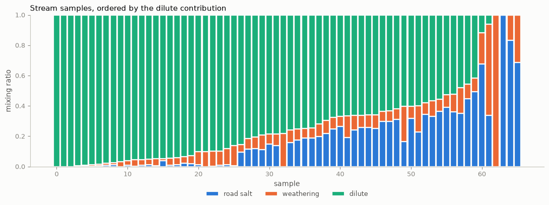
<MixingResult (constrained least squares): 66 samples, mean road salt=18%, weathering=10%, dilute=72%>

road salt     18.2
weathering    10.0
dilute        71.7
Name: mean contribution (%), dtype: float64

Roughly 72% dilute water, 18% road-salt-bearing water, 10% weathering-derived water on average across these samples.

fig, ax = plt.subplots(figsize=(11, 4.2))
plot_ratios(result, ax=ax, order_by=2)
ax.set_title("Stream samples, ordered by the dilute contribution", loc="left", fontsize=11)
fig.tight_layout()

Step 7 — Uncertainty

A number without one is not a result.

mc = monte_carlo_ratios(
    endmembers, samples,
    sd_endmembers=0.20 * endmembers.data,   # how well one sample represents a source
    sd_samples=sigma,
    n_draws=400, seed=0,
)

pd.DataFrame({
    "mean contribution": result.ratios.mean(axis=0).round(3),
    "sd across samples": result.ratios.std(axis=0).round(3),
    "typical 95% width": (mc["upper"] - mc["lower"]).mean(axis=0).round(3),
}, index=endmembers.labels)

	mean contribution	sd across samples	typical 95% width
road salt	0.182	0.211	0.124
weathering	0.100	0.141	0.145
dilute	0.717	0.269	0.125

The typical 95% interval on an individual sample’s fraction is about 0.12 to 0.15 wide. That is the honest precision of a three-end-member separation from six major ions with end-members defined by a single sample each — good enough to say which source dominates, not good enough to argue about five percentage points.

Step 8 — Residuals as chemistry

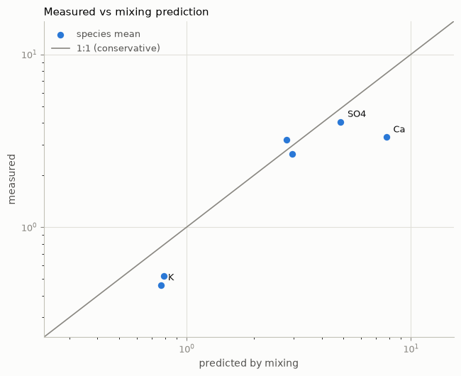
conservative = fit_conservative(endmembers, samples, conservative=["Cl", "Na"])
classify_source_sink(conservative, samples, threshold=0.15)[
    ["mean_measured", "mean_predicted", "relative_departure", "behaviour", "likely_process"]
].round(3)

	mean_measured	mean_predicted	relative_departure	behaviour	likely_process
species
Ca	3.311	7.768	-0.574	sink	calcite precipitation; exchange uptake
Mg	0.524	0.790	-0.337	sink	dolomite precipitation; exchange uptake
Na	2.663	2.953	-0.098	conservative
K	0.461	0.769	-0.400	sink	clay exchange uptake; biological uptake
Cl	3.211	2.793	0.150	conservative
SO4	4.068	4.857	-0.163	sink	sulphate reduction; gypsum precipitation

fig, ax = plt.subplots(figsize=(6.6, 5.4))
plot_measured_vs_predicted(conservative, samples, ax=ax)
fig.tight_layout()

Conclusion, with its limitations

Result. Stream chemistry in Grafton County is well described as a mixture of three waters: dilute precipitation-derived water (about 72% on average), a road-salt-bearing water (18%) and a weathering-derived water (10%). Two components explain 96% of the variance; the first is dilution and the second separates halite from weathering, matching the conceptual model formed before the data were examined. Individual fractions carry 95% intervals about 0.12–0.15 wide.

Limitations, which belong in the same breath:

1. No bicarbonate, so charge balance could not be verified and the weathering end-member is characterised only by its cations.

2. 11% of samples fall outside the mixing hull — a fourth source, or a reaction, that these three end-members do not cover.

3. End-members are single samples, so their uncertainty is assumed rather than measured. With replicates, jackknife_endmembers would measure it instead.

4. Samples span 1990–2021 and many sites. Mixing analysis assumes end-member compositions are constant; over thirty years of changing road-salt application that is doubtful. A per-catchment, per-decade analysis would be more defensible.

5. Nothing here is confirmed independently. The next steps would be saturation indices in PHREEQC, a Na:Cl equivalent ratio test for the halite hypothesis, and a check against the catchment water balance.

Limitation 4 is the one that would most change the answer, and it is the general lesson of this notebook: the hardest assumption in mixing analysis is not the mathematics, it is that the end-members held still.

The template

import mescla as am
from mescla.reactions.residuals import classify_source_sink, fit_conservative
from mescla.uncertainty.montecarlo import monte_carlo_ratios

# 1. Conceptual model first, written down before you look.
# 2. One system, screened.
samples = am.WaterChemistry.from_frame(my_frame)
am.charge_balance_report(samples)

# 3. EMMA: rank from the loadings and the fit, not from one rule.
model = am.EMMA().fit(samples)
model.rank_summary(); model.loadings_frame(); model.diagnostics().to_frame()

# 4. End-members: real waters that bound the data.
model.suggest_endmembers(candidates)
model.hull_fraction(endmembers)          # report it

# 5. Answerable?
am.identifiability_report(endmembers, samples, model.scores_, model.transform(endmembers))

# 6. Ratios, weighted by judgement.
result = am.mixing_ratios(endmembers, samples, sigma=sigma)

# 7. Uncertainty. Always.
monte_carlo_ratios(endmembers, samples, sd_endmembers=..., sd_samples=sigma)

# 8. Residuals as chemistry.
classify_source_sink(fit_conservative(endmembers, samples, ["Cl", "Na"]), samples)

# 9. Conclusion AND limitations, in the same breath.